# Where the data and the theme live. The defaults load from the companion
# site. Set MV_DATA and MV_THEME to local paths to work offline.
mv_data  <- Sys.getenv("MV_DATA",  "https://viz.marginoferrormedia.com/data")
mv_theme <- Sys.getenv("MV_THEME", "https://viz.marginoferrormedia.com/figures/mv-theme.R")Chapter 12: From Data to Story
The code behind every figure in Chapter 12 of Make It Visible, in the order the chapter draws them. Run the first chunk, then any figure. Each chunk stands on its own once the setup chunk has run.
Setup
Loads the theme, the packages, and the chapter’s data.
Code
source(mv_theme)
mv_set_chapter(12)
suppressPackageStartupMessages({ library(tidyverse); library(ggrepel); library(patchwork) })
le <- read_csv(file.path(mv_data, "ch12-life-expectancy.csv"), show_col_types = FALSE)
ag <- read_csv(file.path(mv_data, "ch12-life-expectancy-ages.csv"), show_col_types = FALSE)
cap_theme <- theme(plot.caption = element_text(size = 7.5, hjust = 0, color = mv_ink$mute, family = mv_font()),
                   plot.background = element_rect(fill = mv_ink$canvas, color = NA))
plain_title <- theme(plot.title = element_text(size = rel(1), face = "plain"))
src <- "UN World Population Prospects and Human Mortality Database, via Our World in Data"
peers <- c("Japan", "Australia", "Italy", "Spain", "Sweden", "France", "Canada", "Germany", "United Kingdom")
countries <- le |> filter(!is.na(code), code != "OWID_WRL")
rich <- le |> filter(country %in% c(peers, "United States"), year >= 1960)
Figure 12.1
Life expectancy at birth for every country, 1950 to 2021, one line each. This is an exploration chart. A reader can see that nearly every line rises, that the spread narrowed, and that many lines fall in 2020 and 2021. No single line can be identified. Source: UN World Population Prospects and Human Mortality Database, via Our World in Data.
Code
ggplot(countries, aes(year, life_expectancy, group = country)) +
  geom_line(color = mv_ink$ink, alpha = 0.12, linewidth = 0.4) +
  scale_x_continuous(breaks = seq(1950, 2020, 10)) +
  labs(title = paste0("Life expectancy at birth in ", n_distinct(countries$country), " countries, 1950 to 2021"), x = NULL, y = NULL, caption = mv_source(src)) +
  theme_mv() + plain_title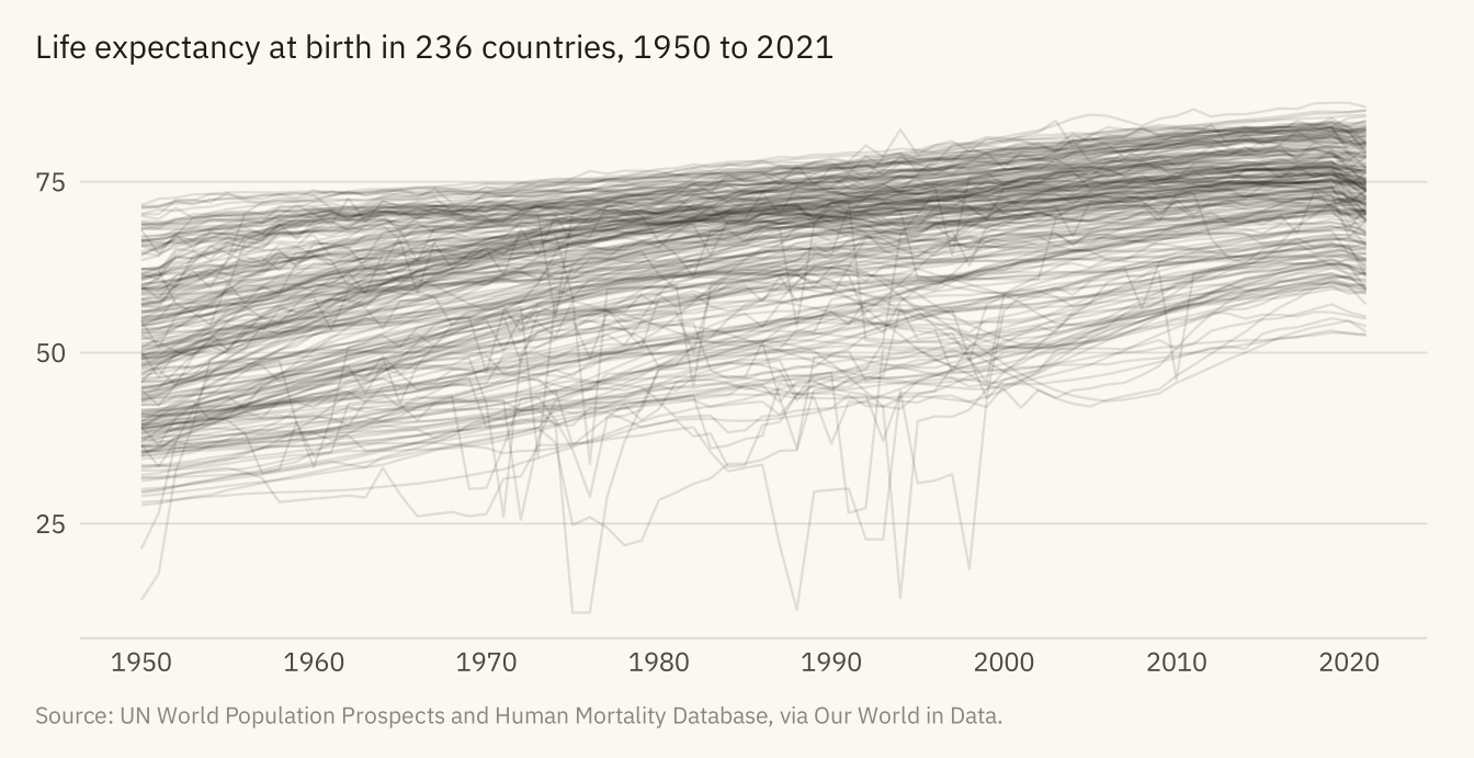
Figure 12.2
Life expectancy at birth in the United States and nine peer countries, 1960 to 2021. The peers are Japan, Australia, Italy, Spain, Sweden, France, Canada, Germany, and the United Kingdom. In 1960 the United States was sixth of the ten. From the late 1980s it has been at the bottom. The gap has widened since. Source: UN World Population Prospects and Human Mortality Database, via Our World in Data.
Code
# Space the end labels by hand: sort by value and push each one down until
# it clears the one above it by 0.7 years.
ends <- rich |> filter(year == 2021) |> arrange(desc(life_expectancy)) |>
  mutate(label_y = life_expectancy)
for (i in seq_len(nrow(ends))[-1]) {
  ends$label_y[i] <- min(ends$label_y[i], ends$label_y[i - 1] - 0.7)
}
ends <- ends |> mutate(is_us = country == "United States",
                       col = if_else(is_us, mv_accent(), mv_ink$mute),
                       sz = if_else(is_us, 3, 2.6))
ggplot(rich, aes(year, life_expectancy, group = country)) +
  geom_line(data = filter(rich, country != "United States"), color = mv_ink$mute, linewidth = 0.7, alpha = 0.7) +
  geom_line(data = filter(rich, country == "United States"), color = mv_accent(), linewidth = 1.2) +
  geom_text(data = ends, aes(x = 2021.6, y = label_y, label = country), color = ends$col,
            size = ends$sz, hjust = 0, family = mv_font()) +
  scale_x_continuous(breaks = seq(1960, 2020, 10), limits = c(1960, 2033), expand = expansion(mult = 0.01)) +
  scale_y_continuous(limits = c(65, 86)) +
  labs(title = "Life expectancy at birth, United States and nine peer countries, 1960 to 2021",
       subtitle = "Years. The United States in black, the nine peers in grey.",
       x = NULL, y = NULL, caption = paste0(mv_source(src), "\nAxis starts at 65 years.")) +
  theme_mv()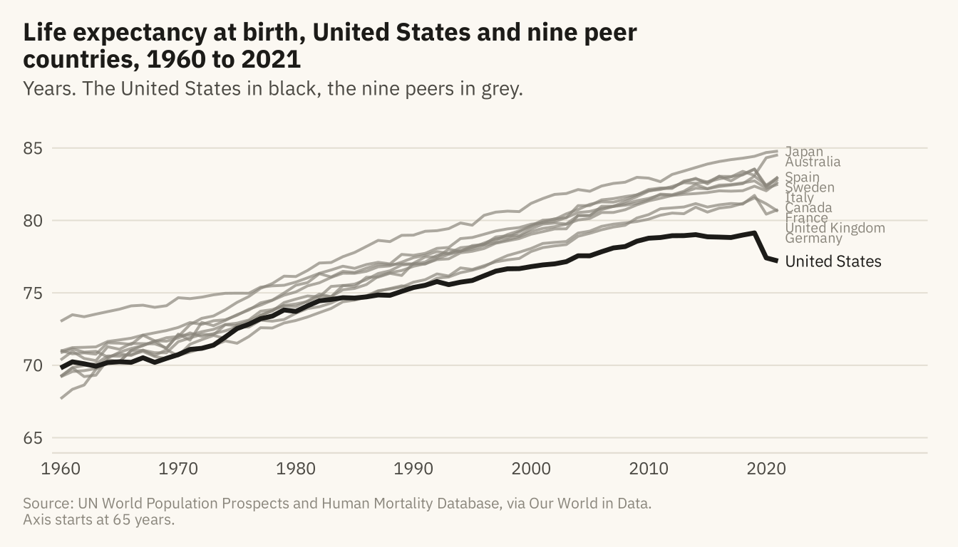
Figure 12.3
The United States minus the median of its nine peers, in years of life expectancy at birth, 1960 to 2021. The gap stayed within about a year of zero through the 1970s. It opened steadily from 1980 and reached three years in 2013. In 2021 it reached 5.7 years. Source: UN World Population Prospects and Human Mortality Database, via Our World in Data.
Code
gap <- rich |> group_by(year) |>
  summarise(us = life_expectancy[country == "United States"],
            peer = median(life_expectancy[country != "United States"]), .groups = "drop") |>
  mutate(gap = us - peer)
ggplot(gap, aes(year, gap)) +
  geom_hline(yintercept = 0, color = mv_ink$ink, linewidth = 0.5) +
  geom_area(fill = mv_accent(), alpha = 0.15) +
  geom_line(color = mv_accent(), linewidth = 1.1) +
  annotate("text", x = 1967, y = 0.6, label = "Level with peers", size = 2.9, family = mv_font(), color = mv_ink$ink2) +
  annotate("text", x = 2019, y = -5.3, label = sprintf("%.1f years\nbehind, 2021", -last(gap$gap)), hjust = 1, size = 2.9,
           family = mv_font(), color = mv_accent(), lineheight = 0.95) +
  scale_x_continuous(breaks = seq(1960, 2020, 10), expand = expansion(mult = 0.01)) +
  scale_y_continuous(limits = c(-6.5, 1.5), breaks = c(-6, -4, -2, 0), labels = \(x) if_else(x == 0, "0", paste0(x, " yrs"))) +
  labs(title = "Life expectancy gap, United States minus peer median, 1960 to 2021",
       subtitle = "United States minus the median of nine peer countries, years at birth",
       x = NULL, y = NULL, caption = mv_source(src)) +
  theme_mv()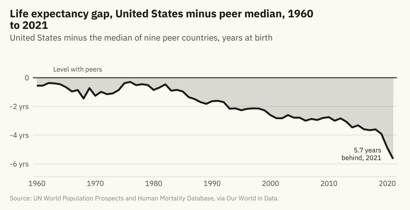
Figure 12.4
The gap between the United States and the peer median in remaining years of life, measured at birth and for people who have already reached 25, 45, and 65, 1960 to 2021. The gap is largest at birth and shrinks with the age already reached. Most of the deficit at birth comes from deaths before 65. Source: UN World Population Prospects and Human Mortality Database, via Our World in Data.
Code
agl <- ag |> filter(country %in% c(peers, "United States"), year >= 1960) |>
  pivot_longer(c(at_birth, at_25, at_45, at_65), names_to = "age", values_to = "le") |>
  group_by(year, age) |>
  summarise(gap = le[country == "United States"] - median(le[country != "United States"]), .groups = "drop") |>
  mutate(age = factor(age, levels = c("at_birth", "at_25", "at_45", "at_65"),
                      labels = c("At birth", "Having reached 25", "Having reached 45", "Having reached 65")))
aend <- agl |> filter(year == 2021) |> arrange(desc(gap)) |>
  mutate(lab = sprintf("%s, %.1f yrs", age, -gap), label_y = gap)
for (i in seq_len(nrow(aend))[-1]) {
  aend$label_y[i] <- min(aend$label_y[i], aend$label_y[i - 1] - 0.45)
}
ggplot(agl, aes(year, gap, color = age)) +
  geom_hline(yintercept = 0, color = mv_ink$ink, linewidth = 0.5) +
  geom_line(linewidth = 0.9) +
  geom_text(data = aend, aes(x = 2021.6, y = label_y, label = lab, color = age),
            hjust = 0, size = 2.7, family = mv_font()) +
  scale_color_manual(values = c(mv_accent(), "#8C3A5E", "#5B6E8C", mv_ink$mute), guide = "none") +
  scale_x_continuous(breaks = seq(1960, 2020, 10), limits = c(1960, 2046), expand = expansion(mult = 0.01)) +
  scale_y_continuous(breaks = c(-6, -4, -2, 0), labels = \(x) if_else(x == 0, "0", paste0(x, " yrs"))) +
  coord_cartesian(clip = "off") +
  labs(title = "Life expectancy gap by age already reached, 1960 to 2021",
       subtitle = "United States minus peer median, years of remaining life, by age already reached",
       x = NULL, y = NULL, caption = mv_source(src)) +
  theme_mv()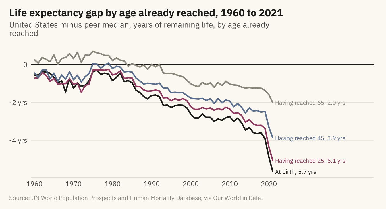
Figure 12.5
The story in three panels. The first shows life expectancy in the United States and its nine peers since 1960. The second shows the gap between the United States and the peer median. The third shows the gap in 2021 by the age already reached. Each panel has one title that states its finding, and the three titles can be read in order as a short paragraph. Source: UN World Population Prospects and Human Mortality Database, via Our World in Data.
Code
s1 <- ggplot(rich, aes(year, life_expectancy, group = country)) +
  geom_line(data = filter(rich, country != "United States"), color = mv_ink$mute, linewidth = 0.5, alpha = 0.7) +
  geom_line(data = filter(rich, country == "United States"), color = mv_accent(), linewidth = 1) +
  scale_x_continuous(breaks = c(1960, 1990, 2020)) +
  scale_y_continuous(limits = c(65, 86), breaks = seq(65, 85, 5), labels = \(x) paste0(x, " yrs")) +
  labs(title = "1. The US fell to the\nbottom of its peers", x = NULL, y = NULL) + theme_mv(base_size = 9) + plain_title
s2 <- ggplot(gap, aes(year, gap)) +
  geom_hline(yintercept = 0, color = mv_ink$ink, linewidth = 0.4) +
  geom_area(fill = mv_accent(), alpha = 0.15) + geom_line(color = mv_accent(), linewidth = 1) +
  scale_x_continuous(breaks = c(1960, 1990, 2020)) +
  scale_y_continuous(limits = c(-6.5, 1.5), breaks = c(-6, -4, -2, 0), labels = \(x) if_else(x == 0, "0", paste0(x, " yrs"))) +
  labs(title = "2. The gap is now\n5.7 years", x = NULL, y = NULL) + theme_mv(base_size = 9) + plain_title
s3 <- ggplot(filter(agl, year == 2021), aes(gap, fct_rev(age))) +
  geom_col(fill = mv_accent(), width = 0.6) +
  geom_text(aes(x = 0, label = sprintf("%.1f yrs", -gap)), hjust = 1.15, size = 2.6, family = mv_font(), color = mv_ink$canvas) +
  scale_x_continuous(limits = c(-6.5, 0), expand = expansion(0), breaks = c(-6, -4, -2, 0),
                     labels = \(x) if_else(x == 0, "0", paste0(x, " yrs"))) +
  labs(title = "3. The gap shrinks with\nthe age already reached", x = NULL, y = NULL) + theme_mv(base_size = 9, grid = "x") + plain_title
s1 + s2 + s3 + plot_annotation(caption = mv_source(src), theme = cap_theme)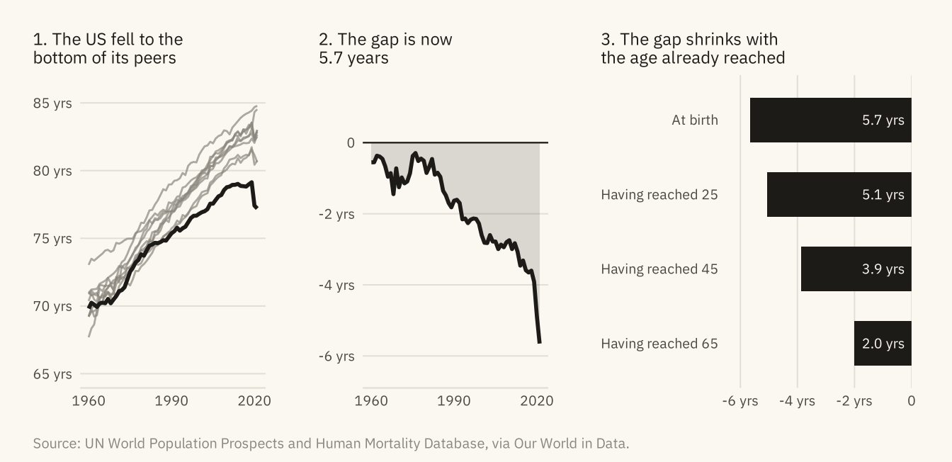
The checklist. Nine questions, with the chapter that explain
Code
tibble::tribble(
  ~Question, ~Chapter,
  "What is counted, and does the title say so?", "3",
  "Does the chart answer one question, and is it the right question?", "1, 4 to 8",
  "Is the encoding as high on the hierarchy as the data allows?", "2",
  "Do bars start at zero, and do truncated axes say why?", "2, 7",
  "Is the comparison fair, and is the window the full one?", "3, 12",
  "Is the unit of analysis stated, and would the other unit change the story?", "5, 8",
  "Is uncertainty shown where it matters?", "10",
  "Does the title state the finding, with one accent and no legend the chart can do without?", "9",
  "Does the caption say what the data cannot show?", "6, 12"
) |> knitr::kable()| Question | Chapter |
|---|---|
| What is counted, and does the title say so? | 3 |
| Does the chart answer one question, and is it the right question? | 1, 4 to 8 |
| Is the encoding as high on the hierarchy as the data allows? | 2 |
| Do bars start at zero, and do truncated axes say why? | 2, 7 |
| Is the comparison fair, and is the window the full one? | 3, 12 |
| Is the unit of analysis stated, and would the other unit change the story? | 5, 8 |
| Is uncertainty shown where it matters? | 10 |
| Does the title state the finding, with one accent and no legend the chart can do without? | 9 |
| Does the caption say what the data cannot show? | 6, 12 |