# Where the data and the theme live. The defaults load from the companion
# site. Set MV_DATA and MV_THEME to local paths to work offline.
mv_data  <- Sys.getenv("MV_DATA",  "https://viz.marginoferrormedia.com/data")
mv_theme <- Sys.getenv("MV_THEME", "https://viz.marginoferrormedia.com/figures/mv-theme.R")Chapter 2: How We See
The code behind every figure in Chapter 2 of Make It Visible, in the order the chapter draws them. Run the first chunk, then any figure. Each chunk stands on its own once the setup chunk has run.
Setup
Loads the theme, the packages, and the chapter’s data.
Code
source(mv_theme)
mv_set_chapter(2)
suppressPackageStartupMessages({ library(tidyverse); library(ggrepel); library(patchwork) })
pm     <- read_csv(file.path(mv_data, "ch02-pm25-exposure.csv"), show_col_types = FALSE)
deaths <- read_csv(file.path(mv_data, "ch02-air-pollution-deaths.csv"), show_col_types = FALSE)
orings <- read_csv(file.path(mv_data, "ch02-orings.csv"), show_col_types = FALSE)
Figure 2.1
O-ring distress on the 23 Space Shuttle flights before Challenger, by temperature at launch. Every flight below 65 degrees showed damage. Flights that share a temperature are stacked so each is visible. The forecast for January 28, 1986 is marked. Source: Dalal, Fowlkes, and Hoadley (1989).
Code
orings_sp <- orings |>
  group_by(temp_f, distress) |>
  mutate(y = distress + (row_number() - (n() + 1) / 2) * 0.17) |>
  ungroup()
ggplot(orings_sp, aes(temp_f, y)) +
  annotate("rect", xmin = 26, xmax = 29, ymin = -0.1, ymax = 2.4, fill = mv_accent(), alpha = 0.25) +
  annotate("text", x = 27.5, y = 2.45, label = "Forecast for launch\nJanuary 28, 1986", vjust = 0,
           size = 2.9, family = mv_font(), color = mv_accent(), lineheight = 0.9) +
  geom_point(size = 2.2, color = mv_ink$ink, alpha = 0.85) +
  scale_x_continuous(limits = c(24, 84), breaks = seq(30, 80, 10),
                     labels = \(x) paste0(x, "°F")) +
  scale_y_continuous(breaks = 0:2, limits = c(-0.15, 2.95)) +
  labs(title = "O-ring distress on 23 Shuttle flights before Challenger, by launch temperature",
       subtitle = "Number of O-rings showing distress per flight, launch temperature in degrees Fahrenheit",
       x = NULL, y = NULL, caption = mv_source("Dalal, Fowlkes, and Hoadley (1989)")) +
  theme_mv()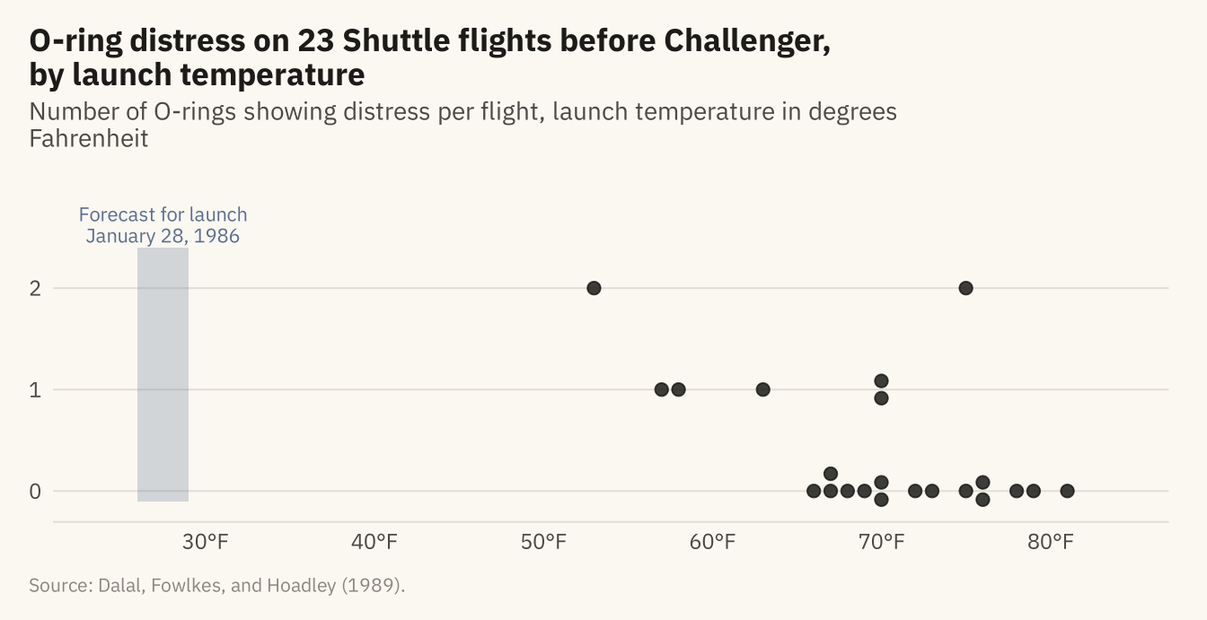
Figure 2.2
The same digits in the same positions, drawn twice. On the left, all digits are one color, and a reader finds the 5s one digit at a time. On the right, the 5s are in a second color. A reader can see them at once, because color is a preattentive feature.
Code
set.seed(42)
grid <- expand_grid(row = 1:5, col = 1:12) |>
  mutate(digit = sample(c(0:4, 6:9), n(), replace = TRUE))
grid$digit[c(27, 40, 56)] <- 5
grid <- grid |> mutate(is5 = digit == 5)

p_plain <- ggplot(grid, aes(col, -row, label = digit)) +
  geom_text(family = mv_font(), size = 4.2, color = mv_ink$ink) +
  labs(title = "Attentive: all digits in one color") + theme_mv_blank(base_size = 10) +
  theme(plot.title = element_text(size = rel(1), face = "plain"))
p_pop <- ggplot(grid, aes(col, -row, label = digit, color = is5)) +
  geom_text(family = mv_font(), size = 4.2, fontface = ifelse(grid$is5, "bold", "plain")) +
  scale_color_manual(values = c(`FALSE` = mv_ink$ink, `TRUE` = "#B3261E"), guide = "none") +
  labs(title = "Preattentive: the 5s in a second color") + theme_mv_blank(base_size = 10) +
  theme(plot.title = element_text(size = rel(1), face = "plain"))
p_plain + p_pop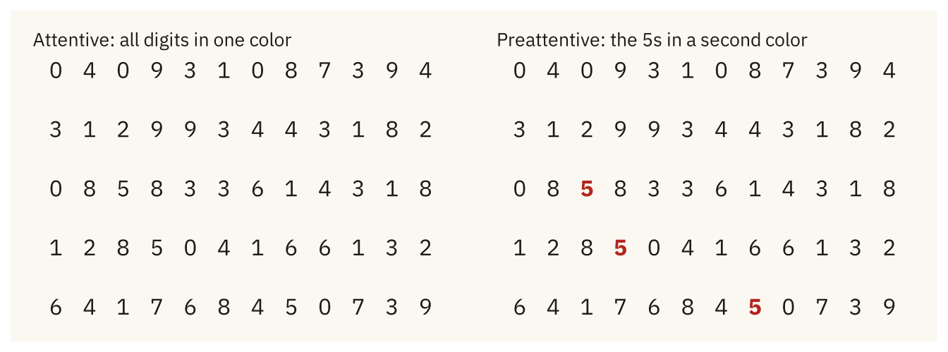
Figure 2.3
Deaths attributed to outdoor PM2.5 in 2015, by World Bank region, as a pie and as a bar chart. In the pie, a reader compares angles. In the bars, a reader compares lengths from a shared baseline, which readers do with less error. Source: State of Global Air, via Our World in Data.
Code
reg <- deaths |>
  filter(year == 2015, !is.na(region)) |>
  group_by(region) |>
  summarise(d = sum(deaths_ambient_pm25, na.rm = TRUE), .groups = "drop") |>
  mutate(region = str_replace(region, " & ", " and "),
         region = fct_reorder(region, d))

pie <- ggplot(reg, aes(x = 1, y = d, fill = region)) +
  geom_col(color = mv_ink$canvas, linewidth = 0.9) +
  coord_polar(theta = "y") +
  scale_fill_manual(values = colorRampPalette(c("#CFC6B2", mv_accent(), "#3A1410"))(7)) +
  labs(fill = NULL, title = "As a pie") +
  guides(fill = guide_legend(ncol = 1, reverse = TRUE)) +
  theme_mv_blank(base_size = 10) +
  theme(legend.position = "bottom", legend.text = element_text(size = rel(0.7)),
        legend.key.size = unit(0.6, "lines"), plot.title = element_text(size = rel(1), face = "plain"))

bar <- ggplot(reg, aes(d, region)) +
  geom_col(fill = mv_accent(), width = 0.7) +
  scale_x_continuous(labels = c("0", "0.75M", "1.5M"),
                     breaks = c(0, 0.75e6, 1.5e6), expand = expansion(mult = c(0, 0.05))) +
  labs(x = NULL, y = NULL, title = "As bars") +
  theme_mv(base_size = 10, grid = "x") +
  theme(plot.title = element_text(size = rel(1), face = "plain"))

pie + bar + plot_layout(widths = c(1, 1)) +
  plot_annotation(caption = mv_source("State of Global Air, via Our World in Data"),
                  theme = theme(plot.caption = element_text(size = 7.5, hjust = 0,
                                color = mv_ink$mute, family = mv_font()),
                                plot.background = element_rect(fill = mv_ink$canvas, color = NA)))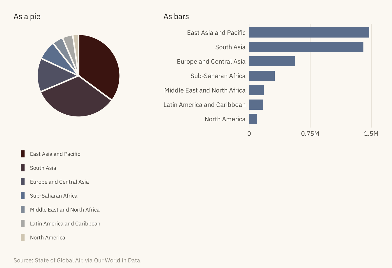
Figure 2.4
Share of all deaths attributed to air pollution in 2017 for eight countries, split by source. In the stacked version, the outdoor segments start at different heights and are hard to compare. In the side by side version, the same segments share a baseline and the reader compares lengths. Source: IHME Global Burden of Disease 2019, via Our World in Data.
Code
eight <- c("India", "Bangladesh", "Nepal", "Egypt", "China", "Nigeria", "Germany", "United States")
src <- deaths |>
  filter(year == 2017, country %in% eight) |>
  select(country, Indoor = share_indoor, Outdoor = share_outdoor) |>
  pivot_longer(-country, names_to = "source", values_to = "share") |>
  mutate(country = factor(country, levels = rev(eight)),
         source = factor(source, levels = c("Outdoor", "Indoor")))

stacked <- ggplot(src, aes(share, country, fill = source)) +
  geom_col(width = 0.7) +
  scale_fill_manual(values = c(Outdoor = mv_accent(), Indoor = mv_ink$mute)) +
  scale_x_continuous(labels = label_percent(scale = 1), expand = expansion(mult = c(0, 0.05))) +
  labs(x = NULL, y = NULL, fill = NULL, title = "Stacked: outdoor and indoor shares in one bar") +
  theme_mv(base_size = 10, grid = "x") +
  theme(plot.title = element_text(size = rel(1), face = "plain"))

dodged <- ggplot(src, aes(share, country, fill = source)) +
  geom_col(width = 0.7, position = position_dodge(width = 0.75)) +
  scale_fill_manual(values = c(Outdoor = mv_accent(), Indoor = mv_ink$mute)) +
  scale_x_continuous(labels = label_percent(scale = 1), expand = expansion(mult = c(0, 0.05))) +
  labs(x = NULL, y = NULL, fill = NULL, title = "Side by side: the same shares on a shared baseline") +
  theme_mv(base_size = 10, grid = "x") +
  theme(plot.title = element_text(size = rel(1), face = "plain"), legend.position = "none")

(stacked / dodged) +
  plot_annotation(caption = mv_source("IHME Global Burden of Disease 2019, via Our World in Data"),
                  theme = theme(plot.caption = element_text(size = 7.5, hjust = 0,
                                color = mv_ink$mute, family = mv_font()),
                                plot.background = element_rect(fill = mv_ink$canvas, color = NA)))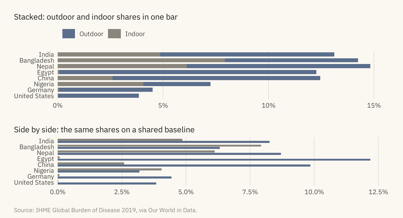
Figure 2.5
Mean annual PM2.5 exposure in 2017 for six countries, as circles scaled by area and as bars. India’s exposure is twelve times that of the United States. In the circles, the ratio looks like three or four times. In the bars, it looks like twelve. Source: World Bank, via Our World in Data.
Code
six <- pm |> filter(year == 2017, country %in% c("India", "Nigeria", "China", "Mexico", "Germany", "United States")) |>
  mutate(country = fct_reorder(country, pm25))

circles <- ggplot(six, aes(x = 1, y = country, size = pm25)) +
  geom_point(color = mv_accent(), alpha = 0.85) +
  scale_size_area(max_size = 12, guide = "none") +
  scale_x_continuous(limits = c(0.5, 1.5)) +
  scale_y_discrete(expand = expansion(add = 0.8)) +
  labs(x = NULL, y = NULL, title = "Area: circles scaled\nto the value") +
  theme_mv_blank(base_size = 10) +
  theme(axis.text.y = element_text(size = rel(0.85), color = mv_ink$ink2),
        plot.title = element_text(size = rel(1), face = "plain"))

bars <- ggplot(six, aes(pm25, country)) +
  geom_col(fill = mv_accent(), width = 0.6) +
  geom_text(aes(label = round(pm25)), hjust = -0.3, size = 3, family = mv_font(), color = mv_ink$ink2) +
  scale_x_continuous(expand = expansion(mult = c(0, 0.15))) +
  labs(x = NULL, y = NULL, title = "Length: bars from\na common baseline") +
  theme_mv(base_size = 10, grid = "none") +
  theme(axis.text.x = element_blank(), axis.text.y = element_blank(),
        plot.title = element_text(size = rel(1), face = "plain"))

circles + bars +
  plot_annotation(caption = mv_source("World Bank, via Our World in Data", "micrograms per cubic meter"),
                  theme = theme(plot.caption = element_text(size = 7.5, hjust = 0,
                                color = mv_ink$mute, family = mv_font()),
                                plot.background = element_rect(fill = mv_ink$canvas, color = NA)))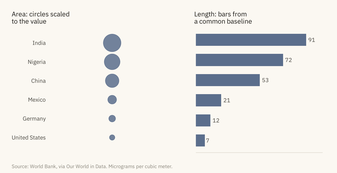
Figure 2.6
PM2.5 exposure for four countries, 1990 to 2017, drawn twice. Left: the points are unconnected and in one color, and a reader sees a cloud. Right: lines connect each country’s points, color separates the countries, and a direct label replaces the legend. Source: World Bank, via Our World in Data.
Code
four <- pm |> filter(country %in% c("India", "China", "Nigeria", "United States"))
ends <- four |> filter(year == 2017)

cloud <- ggplot(four, aes(year, pm25)) +
  geom_point(size = 1.8, color = mv_ink$ink, alpha = 0.7) +
  scale_x_continuous(breaks = c(1990, 2000, 2010, 2017)) +
  labs(x = NULL, y = NULL, title = "Points only, in one color") +
  theme_mv(base_size = 10) + theme(plot.title = element_text(size = rel(1), face = "plain"))

paths <- ggplot(four, aes(year, pm25, color = country)) +
  geom_line(linewidth = 0.9) +
  geom_point(size = 1.4) +
  mv_label_end(ends, aes(label = country, color = country), nudge_x = 1) +
  scale_color_manual(values = c(India = mv_ink$ink, China = mv_accent(),
                                Nigeria = "#2E6B5E", `United States` = "#7A4E8C"), guide = "none") +
  scale_x_continuous(breaks = c(1990, 2000, 2010, 2017), limits = c(1990, 2034)) +
  labs(x = NULL, y = NULL, title = "Lines and color, one per country") +
  theme_mv(base_size = 10) + theme(plot.title = element_text(size = rel(1), face = "plain"))

cloud + paths +
  plot_annotation(caption = mv_source("World Bank, via Our World in Data", "micrograms per cubic meter"),
                  theme = theme(plot.caption = element_text(size = 7.5, hjust = 0,
                                color = mv_ink$mute, family = mv_font()),
                                plot.background = element_rect(fill = mv_ink$canvas, color = NA)))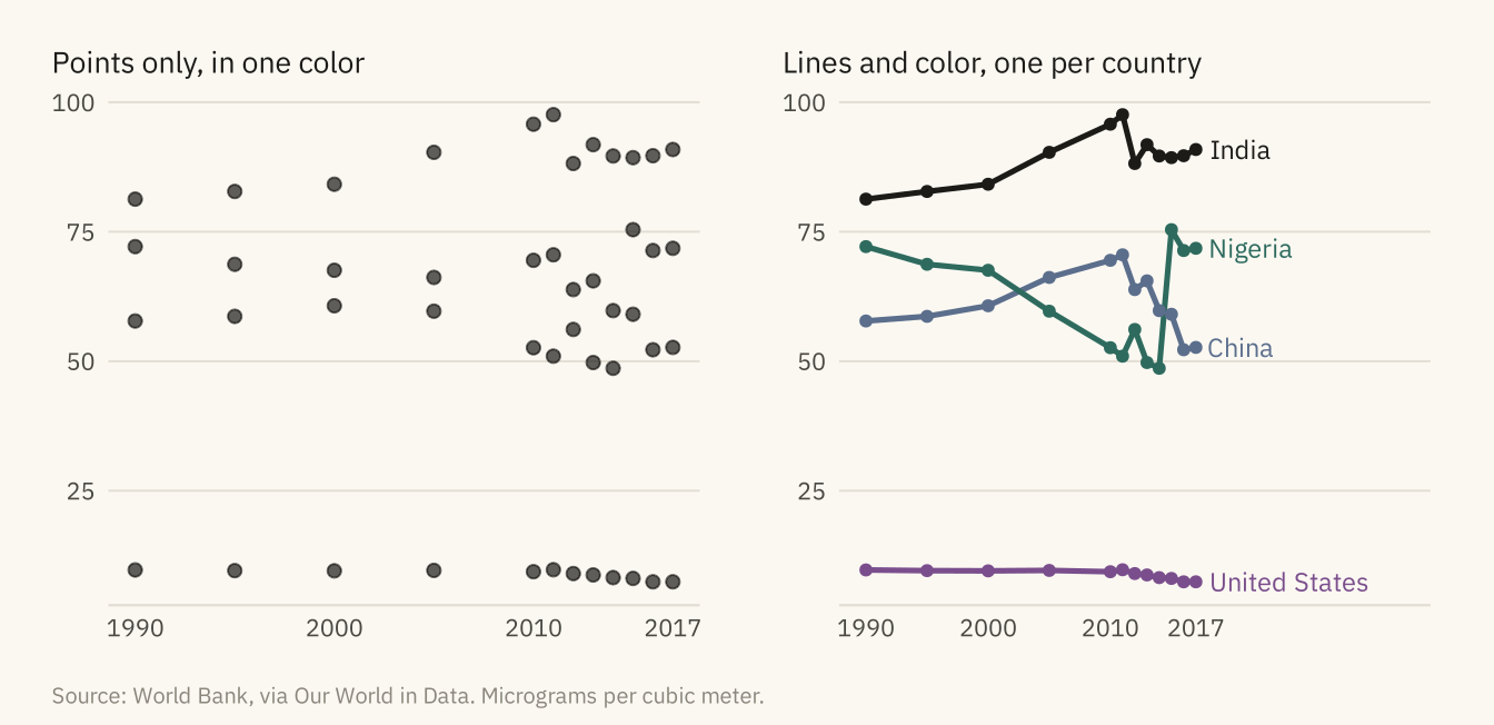
Figure 2.7
The same thirty countries, sorted by PM2.5 exposure in 2017 from low on the left to high on the right, shaded three ways. The rainbow adds boundaries that are not in the data. The single-hue ramp shows a smooth ordering. The diverging ramp does not fit here. Its light middle falls at 55 micrograms, between the 27th and 28th tiles, because the data has no meaningful center. Source: World Bank, via Our World in Data.
Code
thirty <- pm |> filter(year == 2017, !is.na(region)) |>
  arrange(desc(pm25)) |> slice(seq(1, 190, by = 6)) |> slice_head(n = 30) |>
  arrange(pm25) |>
  mutate(rank = row_number())

strip <- function(scale, title) {
  ggplot(thirty, aes(rank, 1, fill = pm25)) +
    geom_tile(color = mv_ink$canvas, linewidth = 0.4) + scale +
    labs(title = title, x = NULL, y = NULL) +
    theme_mv_blank(base_size = 10) +
    theme(legend.position = "none", plot.title = element_text(size = rel(0.95), face = "plain"),
          plot.margin = margin(4, 8, 4, 8))
}
strip(scale_fill_gradientn(colors = rainbow(7)), "Rainbow: several hues across the range") /
strip(scale_fill_gradientn(colors = colorRampPalette(c("#CFC6B2", mv_accent(), "#2A3A52"))(9)),
      "Sequential: one hue, light to dark") /
strip(scale_fill_gradientn(colors = colorRampPalette(c("#B8862B", "#E8E2D4", "#2A3A52"))(9)),
      "Diverging: two hues meeting at a middle value") +
  plot_annotation(caption = mv_source("World Bank, via Our World in Data"),
                  theme = theme(plot.caption = element_text(size = 7.5, hjust = 0,
                                color = mv_ink$mute, family = mv_font()),
                                plot.background = element_rect(fill = mv_ink$canvas, color = NA)))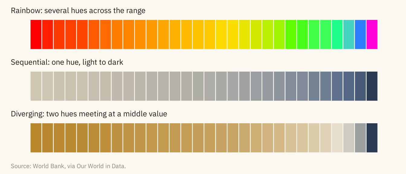
Figure 2.8
PM2.5 exposure in India, 1990 to 2017, drawn twice. Left: the vertical axis starts at 80 and the rise from 1990 to 2017 looks about eightfold. Right: the axis starts at zero and the rise is 12 percent. Both panels use the same numbers. Only the right one lets the reader judge the size of the change. Source: World Bank, via Our World in Data.
Code
india <- pm |> filter(country == "India")
trunc <- ggplot(india, aes(year, pm25)) +
  geom_col(fill = mv_accent(), width = 1.6) +
  coord_cartesian(ylim = c(80, 100)) +
  scale_y_continuous(breaks = seq(80, 100, 5)) +
  scale_x_continuous(breaks = c(1990, 2000, 2010, 2017)) +
  labs(x = NULL, y = NULL, title = "Axis starts at 80") +
  theme_mv(base_size = 10) + theme(plot.title = element_text(size = rel(1), face = "plain"))
full <- ggplot(india, aes(year, pm25)) +
  geom_col(fill = mv_accent(), width = 1.6) +
  scale_y_continuous(limits = c(0, 100), expand = expansion(0)) +
  scale_x_continuous(breaks = c(1990, 2000, 2010, 2017)) +
  labs(x = NULL, y = NULL, title = "Axis starts at zero") +
  theme_mv(base_size = 10) + theme(plot.title = element_text(size = rel(1), face = "plain"))
trunc + full +
  plot_annotation(caption = mv_source("World Bank, via Our World in Data", "micrograms per cubic meter"),
                  theme = theme(plot.caption = element_text(size = 7.5, hjust = 0,
                                color = mv_ink$mute, family = mv_font()),
                                plot.background = element_rect(fill = mv_ink$canvas, color = NA)))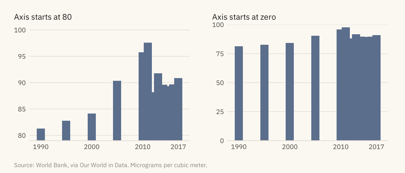
Figure 2.9
The six-country exposure chart drawn with spreadsheet defaults and again with the non-data ink removed. The data is identical in both. Source: World Bank, via Our World in Data.
Code
junk <- ggplot(six, aes(country, pm25, fill = country)) +
  geom_col(color = "black", width = 0.75) +
  scale_fill_manual(values = c("#4472C4", "#ED7D31", "#A5A5A5", "#FFC000", "#5B9BD5", "#70AD47")) +
  scale_y_continuous(breaks = seq(0, 100, 10), minor_breaks = seq(0, 100, 5)) +
  labs(x = "Country", y = "PM2.5 (ug/m3)", fill = "Country", title = "PM2.5 by Country") +
  theme_gray(base_size = 9) +
  theme(panel.grid.major = element_line(color = "grey40"), panel.grid.minor = element_line(color = "grey60"),
        panel.border = element_rect(fill = NA, color = "black", linewidth = 1),
        plot.background = element_rect(fill = "#DDEBF7", color = "black"),
        axis.text.x = element_text(angle = 45, hjust = 1),
        plot.title = element_text(face = "bold.italic", hjust = 0.5))
clean <- ggplot(six, aes(pm25, country)) +
  geom_col(fill = mv_accent(), width = 0.6) +
  geom_text(aes(label = round(pm25)), hjust = -0.3, size = 3, family = mv_font(), color = mv_ink$ink2) +
  scale_x_continuous(expand = expansion(mult = c(0, 0.2))) +
  labs(x = NULL, y = NULL, title = "Annual PM2.5 exposure, 2017",
       subtitle = "Micrograms per cubic meter") +
  theme_mv(base_size = 10, grid = "none") +
  theme(axis.text.x = element_blank(), plot.title = element_text(size = rel(1)))
junk + clean +
  plot_annotation(caption = mv_source("World Bank, via Our World in Data"),
                  theme = theme(plot.caption = element_text(size = 7.5, hjust = 0,
                                color = mv_ink$mute, family = mv_font()),
                                plot.background = element_rect(fill = mv_ink$canvas, color = NA)))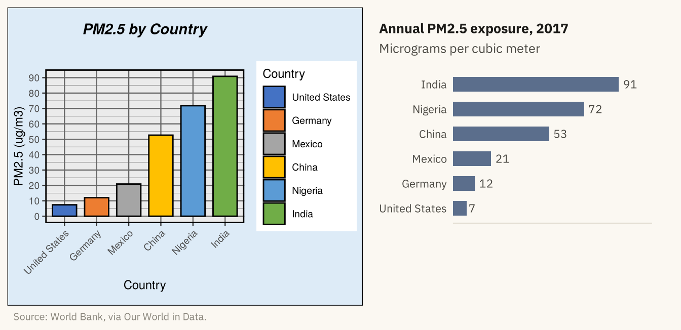
Figure 2.10
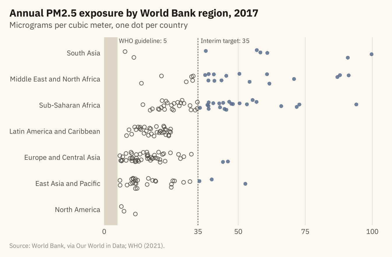
Population-weighted annual PM2.5 exposure in 2017, one dot per country, grouped by World Bank region. The shaded band is the WHO guideline of 5 micrograms per cubic meter. No country meets it. The filled dots in the accent color, to the right of the dashed line, are the 48 countries above 35, the WHO’s loosest interim target. Source: World Bank, via Our World in Data; WHO Global Air Quality Guidelines (2021).
Code
now <- pm |> filter(year == 2017, !is.na(region)) |>
  mutate(region = str_replace(region, " & ", " and "),
         region = fct_reorder(region, pm25, .fun = median),
         over35 = pm25 > 35)
set.seed(7)
ggplot(now, aes(pm25, region)) +
  annotate("rect", xmin = 0, xmax = 5, ymin = -Inf, ymax = Inf, fill = "#D9D2C2", alpha = 0.9) +
  annotate("text", x = 5.5, y = Inf, label = "WHO guideline: 5", hjust = 0, vjust = 1.3,
           size = 2.8, family = mv_font(), color = mv_ink$ink2) +
  geom_vline(xintercept = 35, linetype = "22", color = mv_ink$ink2, linewidth = 0.4) +
  annotate("text", x = 36, y = Inf, label = "Interim target: 35", hjust = 0, vjust = 1.3,
           size = 2.8, family = mv_font(), color = mv_ink$ink2) +
  geom_jitter(aes(color = over35, shape = over35), height = 0.2, width = 0, size = 1.9,
              alpha = 0.85, stroke = 0.6) +
  scale_color_manual(values = c(`FALSE` = mv_ink$ink2, `TRUE` = mv_accent()), guide = "none") +
  scale_shape_manual(values = c(`FALSE` = 1, `TRUE` = 16), guide = "none") +
  scale_x_continuous(expand = expansion(mult = c(0, 0.03)), breaks = c(0, 35, 50, 75, 100)) +
  labs(title = "Annual PM2.5 exposure by World Bank region, 2017",
       subtitle = "Micrograms per cubic meter, one dot per country",
       x = NULL, y = NULL,
       caption = mv_source("World Bank, via Our World in Data; WHO (2021)")) +
  theme_mv(grid = "x")