# Where the data and the theme live. The defaults load from the companion
# site. Set MV_DATA and MV_THEME to local paths to work offline.
mv_data  <- Sys.getenv("MV_DATA",  "https://viz.marginoferrormedia.com/data")
mv_theme <- Sys.getenv("MV_THEME", "https://viz.marginoferrormedia.com/figures/mv-theme.R")Chapter 8: Place
The code behind every figure in Chapter 8 of Make It Visible, in the order the chapter draws them. Run the first chunk, then any figure. Each chunk stands on its own once the setup chunk has run.
Setup
Loads the theme, the packages, and the chapter’s data.
Code
source(mv_theme)
mv_set_chapter(8)
suppressPackageStartupMessages({ library(tidyverse); library(ggrepel); library(patchwork); library(sf) })
sf_use_s2(FALSE)
co  <- st_read(file.path(mv_data, "ch08-counties.geojson"), quiet = TRUE) |>
  mutate(fips = if_else(fips == "46113", "46102", fips)) |>  # Shannon County, SD was renamed Oglala Lakota in 2015
  filter(fips != "51515")                                      # Bedford City, VA merged into Bedford County in 2013
acs <- read_csv(file.path(mv_data, "ch08-county-acs-2015.csv"), show_col_types = FALSE)
na_grey <- "#B8B3A8"
rent <- read_csv(file.path(mv_data, "ch08-bay-area-rentals.csv"), show_col_types = FALSE)
cty <- co |> left_join(acs, by = "fips")
states <- cty |> group_by(state_fips) |> summarise(geometry = st_union(geometry), .groups = "drop")
albers <- 5070
cap_theme <- theme(plot.caption = element_text(size = 7.5, hjust = 0, color = mv_ink$mute, family = mv_font()),
                   plot.background = element_rect(fill = mv_ink$canvas, color = NA))
plain_title <- theme(plot.title = element_text(size = rel(1), face = "plain"))
src <- "ACS 2011 to 2015; US Census Bureau boundaries"
theme_map <- function(base_size = 11) theme_mv_blank(base_size) + theme(legend.position = "bottom", legend.key.width = unit(1.6, "lines"), legend.key.height = unit(0.5, "lines"))
Figure 8.1
Share of children under 18 living in poverty by county, 2011 to 2015 average. Counties are shaded in six classes by quantile, so each class holds a sixth of counties. The highest rates are in the Deep South, the Mississippi Delta, Appalachia, the Texas border, and reservation counties in the Dakotas and the Southwest. Source: American Community Survey 2011 to 2015; county boundaries from the US Census Bureau.
Code
cty <- cty |> mutate(cp_class = cut(child_poverty, breaks = quantile(child_poverty, probs = seq(0, 1, 1/6), na.rm = TRUE),
                                    include.lowest = TRUE, dig.lab = 3))
ggplot(cty) +
  geom_sf(aes(fill = cp_class), color = mv_ink$canvas, linewidth = 0.05) +
  geom_sf(data = states, fill = NA, color = mv_ink$canvas, linewidth = 0.35) +
  scale_fill_manual(values = mv_ramp_seq(6), name = "Child poverty rate (%)", na.value = na_grey,
                    labels = \(x) str_replace_all(x, c("\\[" = "", "\\(" = "", "\\]" = "", "," = " to "))) +
  coord_sf(crs = albers, default_crs = 4326) +
  guides(fill = guide_legend(nrow = 1, label.position = "bottom", title.position = "top")) +
  labs(title = "Child poverty rate by county, 2011 to 2015",
       subtitle = "Share of children under 18 below the poverty line, five-year average",
       caption = mv_source(src)) +
  theme_map()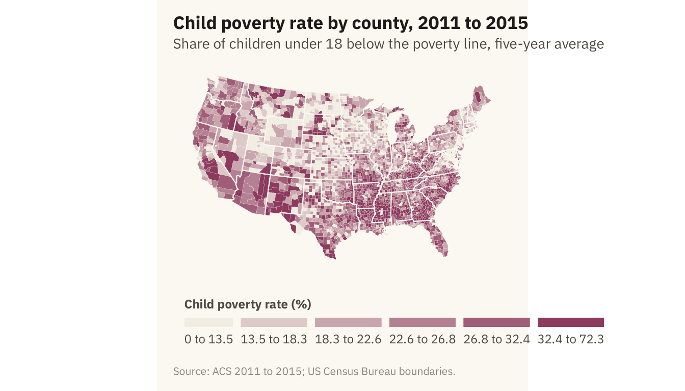
Figure 8.2
The child poverty map in the Albers equal-area projection (left) and in Mercator (right). Mercator enlarges the northern states. The counties of the northern plains, which have few people and mostly low poverty rates, take up more of the page than their true area. Source: American Community Survey 2011 to 2015.
Code
pm <- function(crs, title) {
  ggplot(cty) + geom_sf(aes(fill = cp_class), color = NA) +
    geom_sf(data = states, fill = NA, color = mv_ink$canvas, linewidth = 0.25) +
    scale_fill_manual(values = mv_ramp_seq(6), guide = "none", na.value = na_grey) +
    coord_sf(crs = crs, default_crs = 4326) +
    labs(title = title) + theme_map(base_size = 10) + plain_title
}
pm(albers, "Albers equal-area") + pm(3857, "Mercator") + plot_annotation(caption = mv_source(src), theme = cap_theme)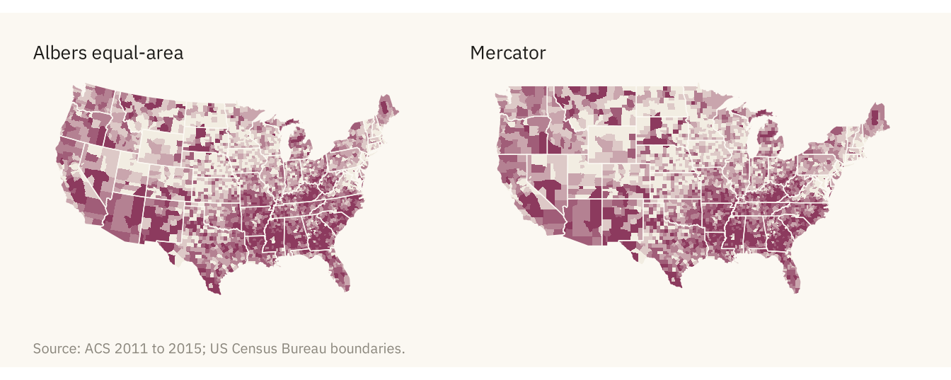
Figure 8.3
Child poverty by county with three rules for class breaks. Equal intervals cut the range into even steps, and most counties fall in the first two classes. Quantiles put a sixth of counties in each class and show the full spread. A single break at the national rate of 22 percent shows one comparison only. Source: American Community Survey 2011 to 2015.
Code
nat_cp <- 22
cty <- cty |> mutate(
  cp_equal = cut(child_poverty, breaks = seq(0, 80, length.out = 7), include.lowest = TRUE),
  cp_two = if_else(child_poverty > nat_cp, "Above the national rate", "At or below"))
pe <- ggplot(cty) + geom_sf(aes(fill = cp_equal), color = NA) +
  geom_sf(data = states, fill = NA, color = mv_ink$canvas, linewidth = 0.25) +
  scale_fill_manual(values = mv_ramp_seq(6), guide = "none", na.value = na_grey) +
  coord_sf(crs = albers, default_crs = 4326) + labs(title = "Equal intervals") + theme_map(base_size = 10) + plain_title
pq <- ggplot(cty) + geom_sf(aes(fill = cp_class), color = NA) +
  geom_sf(data = states, fill = NA, color = mv_ink$canvas, linewidth = 0.25) +
  scale_fill_manual(values = mv_ramp_seq(6), guide = "none", na.value = na_grey) +
  coord_sf(crs = albers, default_crs = 4326) + labs(title = "Quantiles") + theme_map(base_size = 10) + plain_title
pt <- ggplot(cty) + geom_sf(aes(fill = cp_two), color = NA) +
  geom_sf(data = states, fill = NA, color = mv_ink$canvas, linewidth = 0.25) +
  scale_fill_manual(values = c(`Above the national rate` = mv_accent(), `At or below` = "#E8E2D6"), guide = "none", na.value = na_grey) +
  coord_sf(crs = albers, default_crs = 4326) + labs(title = "Above or below 22%") + theme_map(base_size = 10) + plain_title
pe + pq + pt + plot_annotation(caption = mv_source(src), theme = cap_theme)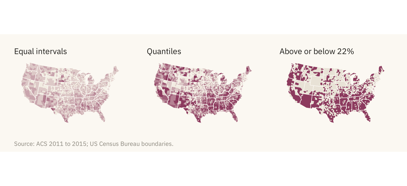
Figure 8.4
Number of children in poverty by county, one circle per county sized by the count. The five largest counts are labeled. Los Angeles County alone has more poor children than 42 of the 48 contiguous states. Most of the large circles are in metropolitan counties, which sit in the middle classes of the rate map. Source: American Community Survey 2011 to 2015.
Code
cent <- cty |> filter(!is.na(child_poverty)) |>
  mutate(poor_children = pop * 0.23 * child_poverty / 100) |>
  st_point_on_surface() |>
  st_transform(albers)
big <- cent |> slice_max(poor_children, n = 5) |> mutate(label = str_remove(county, " County"),
                                                         x = st_coordinates(geometry)[, 1], y = st_coordinates(geometry)[, 2]) |> st_drop_geometry()
ggplot() +
  geom_sf(data = states, fill = "#F2EDE2", color = mv_ink$canvas, linewidth = 0.35) +
  geom_sf(data = cent, aes(size = poor_children), color = mv_accent(), alpha = 0.45, shape = 16) +
  geom_text_repel(data = big, aes(x, y, label = label),
                  size = 3, family = mv_font(), color = mv_ink$ink, bg.color = mv_ink$canvas, bg.r = 0.12,
                  min.segment.length = 0, segment.color = mv_ink$ink, box.padding = 0.8, point.padding = 1.5, seed = 8) +
  scale_size_area(max_size = 16, breaks = c(25000, 100000, 300000), labels = label_comma(), name = "Children in poverty") +
  coord_sf(crs = albers) +
  labs(title = "Number of children in poverty by county,\n2011 to 2015",
       subtitle = "Estimated number of children under 18\nbelow the poverty line",
       caption = "Source: ACS 2011 to 2015; US Census Bureau boundaries.\nChildren estimated as 23 percent of county population.") +
  theme_map() + theme(legend.key.height = unit(1.4, "lines"))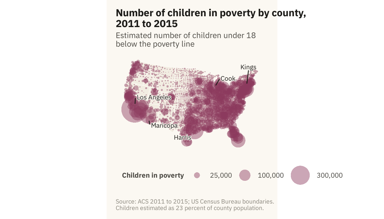
Figure 8.5
Counties sorted by land area, grouped into ten bins of about 310 counties each. The largest tenth of counties by area holds 18 percent of the population and covers 40 percent of the map. The smallest tenth holds 11 percent of the population on 2 percent of the land. Source: American Community Survey 2011 to 2015; areas from county boundaries.
Code
cty_area <- cty |> mutate(area = as.numeric(st_area(st_transform(geometry, albers)))) |> st_drop_geometry() |>
  filter(!is.na(pop)) |> arrange(desc(area)) |>
  mutate(decile = ntile(area, 10), decile = 11 - decile) |>
  group_by(decile) |> summarise(area = sum(area), pop = sum(pop), .groups = "drop") |>
  mutate(`Share of map` = area / sum(area), `Share of people` = pop / sum(pop)) |>
  pivot_longer(c(`Share of map`, `Share of people`), names_to = "what", values_to = "share") |>
  mutate(decile = factor(decile, labels = c("Largest\ntenth", paste0(2:9), "Smallest\ntenth")))
ggplot(cty_area, aes(decile, share, fill = what)) +
  geom_col(position = position_dodge(width = 0.7), width = 0.65) +
  scale_fill_manual(values = c(`Share of map` = mv_ink$mute, `Share of people` = mv_accent()), name = NULL) +
  scale_y_continuous(labels = label_percent(), expand = expansion(mult = c(0, 0.05))) +
  labs(title = "Share of map area and share of population by county size",
       subtitle = "Counties grouped by land area, from largest to smallest tenth",
       x = NULL, y = NULL, caption = mv_source(src)) +
  theme_mv() + theme(axis.text.x = element_text(size = rel(0.8), lineheight = 0.9))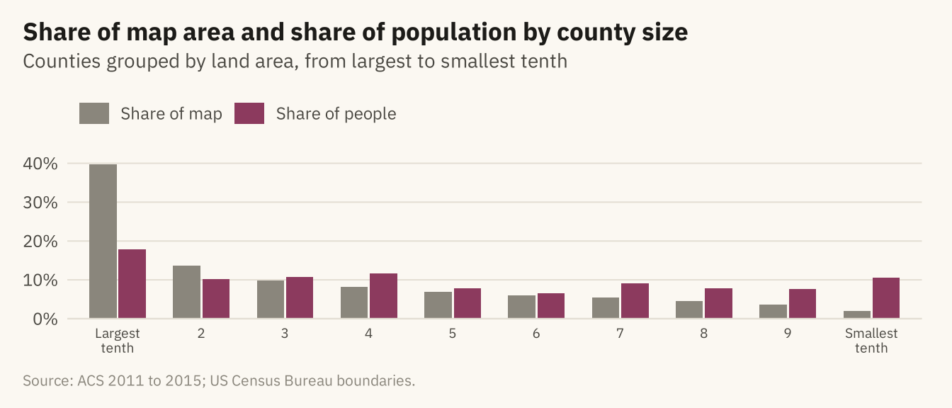
Figure 8.6
Child poverty rate by state on a tile grid. Each state is one square, placed near its geographic position. In the grid, Rhode Island and Texas have the same space, so the small Northeastern states are easy to read. State shapes and some adjacencies are lost. Source: American Community Survey 2011 to 2015, counties aggregated with population weights.
Code
grid <- tribble(
  ~st, ~col, ~row,
  "ME",11,1, "WI",6,2, "VT",10,2, "NH",11,2, "WA",1,3, "ID",2,3, "MT",3,3, "ND",4,3, "MN",5,3, "IL",6,3, "MI",7,3, "NY",9,3, "MA",10,3, "RI",11,3,
  "OR",1,4, "NV",2,4, "WY",3,4, "SD",4,4, "IA",5,4, "IN",6,4, "OH",7,4, "PA",8,4, "NJ",9,4, "CT",10,4,
  "CA",1,5, "UT",2,5, "CO",3,5, "NE",4,5, "MO",5,5, "KY",6,5, "WV",7,5, "VA",8,5, "MD",9,5, "DE",10,5,
  "AZ",2,6, "NM",3,6, "KS",4,6, "AR",5,6, "TN",6,6, "NC",7,6, "SC",8,6, "DC",9,6,
  "OK",4,7, "LA",5,7, "MS",6,7, "AL",7,7, "GA",8,7, "TX",4,8, "FL",8,8)
abbr <- c(setNames(state.abb, state.name), "District of Columbia" = "DC")
st_cp <- acs |> mutate(st = abbr[state]) |> filter(!is.na(st), !is.na(child_poverty)) |>
  group_by(st) |> summarise(cp = weighted.mean(child_poverty, pop), .groups = "drop") |>
  right_join(grid, by = "st")
ggplot(st_cp, aes(col, -row, fill = cp)) +
  geom_tile(color = mv_ink$canvas, linewidth = 1.5, width = 0.95, height = 0.95) +
  geom_text(aes(label = st, color = cp > 24), size = 3, family = mv_font(), fontface = "bold") +
  scale_color_manual(values = c(`TRUE` = mv_ink$canvas, `FALSE` = mv_ink$ink), guide = "none") +
  scale_fill_gradientn(colors = mv_ramp_seq(9), name = "Child poverty rate (%)") +
  coord_equal() +
  labs(title = "Child poverty rate by state, 2011 to 2015",
       subtitle = "Share of children below the poverty line,\ncounty data weighted by population",
       caption = mv_source(src)) +
  theme_map() + theme(legend.key.width = unit(2, "lines"))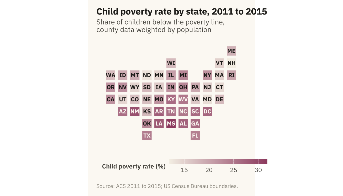
Figure 8.7
Craigslist rental listings in the San Francisco Bay Area with coordinates, 2001 to 2018. Left, every listing as a point colored by asking rent. Right, listings grouped into hexagons, each shaded by its median rent. The hexagons do not overlap, and their shading shows that rent falls with distance from San Francisco and the Peninsula. Source: Pennington (2018), via TidyTuesday.
Code
bay_fips <- c("06001", "06013", "06041", "06055", "06075", "06081", "06085", "06087", "06095", "06097")
bay <- co |> filter(fips %in% bay_fips)
r2 <- rent |> filter(lon > -123, lon < -121.5, lat > 37, lat < 38.6)
pts <- ggplot() +
  geom_sf(data = bay, fill = "#F2EDE2", color = mv_ink$canvas, linewidth = 0.4) +
  geom_point(data = r2, aes(lon, lat, color = price), size = 0.6, alpha = 0.6) +
  scale_color_gradientn(colors = mv_ramp_seq(9), trans = "log10", limits = c(800, 8000), oob = scales::squish,
                        breaks = c(1000, 3000, 8000), labels = c("$1k", "$3k", "$8k"), name = "Asking rent") +
  coord_sf(xlim = c(-123, -121.5), ylim = c(37, 38.6), default_crs = 4326) +
  labs(title = "Every listing") + theme_map(base_size = 10) + plain_title + theme(legend.key.width = unit(1.4, "lines"))
hx <- ggplot() +
  geom_sf(data = bay, fill = "#F2EDE2", color = mv_ink$canvas, linewidth = 0.4) +
  stat_summary_hex(data = r2, aes(lon, lat, z = price), fun = median, bins = 28, color = mv_ink$canvas, linewidth = 0.2) +
  scale_fill_gradientn(colors = mv_ramp_seq(9), trans = "log10", limits = c(800, 8000), oob = scales::squish,
                       breaks = c(1000, 3000, 8000), labels = c("$1k", "$3k", "$8k"), name = "Median rent") +
  coord_sf(xlim = c(-123, -121.5), ylim = c(37, 38.6), default_crs = 4326) +
  labs(title = "Median rent by hexagon") + theme_map(base_size = 10) + plain_title + theme(legend.key.width = unit(1.4, "lines"))
pts + hx + plot_annotation(caption = mv_source("Pennington (2018), via TidyTuesday"), theme = cap_theme)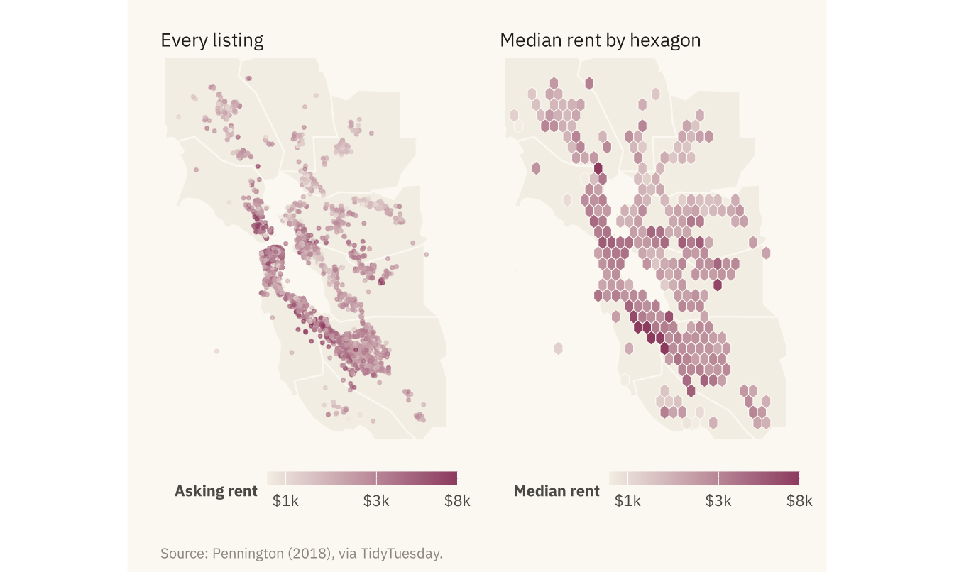
Figure 8.8
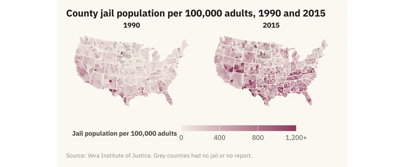
County jail population per 100,000 adults in 1990 and 2015 on the same color scale. Rates rose across the South over the period. The rural counties of Kentucky, Virginia, Tennessee, and Louisiana rose most. Counties with no jail or no report are grey, 187 in 1990 and 175 in 2015. Source: Vera Institute of Justice, Incarceration Trends; boundaries from the US Census Bureau.
Code
jl <- cty |> select(fips, jail_rate_1990, jail_rate_2015) |>
  pivot_longer(c(jail_rate_1990, jail_rate_2015), names_to = "year", values_to = "rate", names_prefix = "jail_rate_") |>
  mutate(rate = if_else(rate <= 0, NA, rate), rate_c = pmin(rate, 1200))
ggplot(jl) +
  geom_sf(aes(fill = rate_c), color = NA) +
  geom_sf(data = states, fill = NA, color = mv_ink$canvas, linewidth = 0.25) +
  facet_wrap(~ year) +
  scale_fill_gradientn(colors = mv_ramp_seq(9), na.value = na_grey, limits = c(0, 1200),
                       breaks = c(0, 400, 800, 1200), labels = c("0", "400", "800", "1,200+"), name = "Jail population per 100,000 adults") +
  coord_sf(crs = albers, default_crs = 4326) +
  labs(title = "County jail population per 100,000 adults, 1990 and 2015", caption = mv_source("Vera Institute of Justice", "grey counties had no jail or no report")) +
  theme_map(base_size = 10) + theme(strip.text = element_text(hjust = 0.5), legend.key.width = unit(2, "lines"))