# Where the data and the theme live. The defaults load from the companion
# site. Set MV_DATA and MV_THEME to local paths to work offline.
mv_data  <- Sys.getenv("MV_DATA",  "https://viz.marginoferrormedia.com/data")
mv_theme <- Sys.getenv("MV_THEME", "https://viz.marginoferrormedia.com/figures/mv-theme.R")Chapter 1: Why We Visualize
The code behind every figure in Chapter 1 of Make It Visible, in the order the chapter draws them. Run the first chunk, then any figure. Each chunk stands on its own once the setup chunk has run.
Setup
Loads the theme, the packages, and the chapter’s data.
Code
source(mv_theme)
mv_set_chapter(1)
suppressPackageStartupMessages({
  library(tidyverse)
  library(ggrepel)
})
world <- read_csv(file.path(mv_data, "ch01-world-under5-since-1800.csv"), show_col_types = FALSE)
u5    <- read_csv(file.path(mv_data, "ch01-under5-by-country.csv"), show_col_types = FALSE) |>
  filter(year >= 1960)
Figure 1.1
Florence Nightingale’s diagram of mortality in the British army, April 1854 to March 1856, redrawn from her data. Each wedge is one month, and its area is the annualized death rate per 1,000 soldiers. In nearly every month, deaths from preventable disease (dark red) are several times deaths from wounds (black). The right-hand circle covers the year after sanitary reforms began in March 1855, and it is smaller. Source: Nightingale (1858), via the HistData package.
Code
library(HistData)

nightingale <- HistData::Nightingale |>
  mutate(Regime = if_else(Date < as.Date("1855-04-01"), "Before", "After"),
         Month = factor(format(Date, "%b"),
                        levels = c("Apr","May","Jun","Jul","Aug","Sep",
                                   "Oct","Nov","Dec","Jan","Feb","Mar"))) |>
  select(Month, Regime, Disease = Disease.rate, Wounds = Wounds.rate, Other = Other.rate) |>
  pivot_longer(c(Disease, Wounds, Other), names_to = "cause", values_to = "rate") |>
  mutate(
    cause  = factor(cause, levels = c("Disease", "Wounds", "Other")),
    Regime = factor(Regime, levels = c("Before", "After"),
                    labels = c("April 1854 to March 1855, before the reforms",
                               "April 1855 to March 1856, after the reforms"))
  ) |>
  arrange(Regime, Month, desc(rate))

# Nightingale drew each cause from the center, not stacked, with the area of
# each wedge proportional to the rate. A square-root radius keeps area honest.
ggplot(nightingale, aes(x = Month, y = rate, fill = cause)) +
  geom_col(position = "identity", width = 1, color = mv_ink$canvas, linewidth = 0.3) +
  coord_polar(start = 0) +
  scale_y_sqrt() +
  scale_fill_manual(values = c(Disease = mv_accent(), Wounds = mv_ink$ink, Other = mv_ink$mute),
                    labels = c("Preventable disease", "Wounds", "Other causes")) +
  facet_wrap(~ Regime, ncol = 2) +
  labs(fill = NULL, x = NULL, y = NULL) +
  theme_mv(grid = "none") +
  theme(axis.text.y = element_blank(), legend.position = "bottom",
        axis.text.x = element_text(size = rel(0.7), color = mv_ink$mute),
        strip.text = element_text(hjust = 0.5))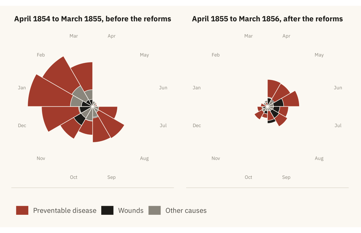
Figure 1.2
Share of children worldwide who died before their fifth birthday, 1800 to 2017. The decline is slow through the nineteenth century, steep from about 1920, and steady after 1960. Source: Gapminder and World Bank, compiled by Our World in Data.
Code
marks <- world |> filter(year %in% c(1800, 1900, 1960, 2017))

ggplot(world, aes(year, share_dying_pct)) +
  geom_area(fill = mv_accent(), alpha = 0.12) +
  geom_line(color = mv_accent(), linewidth = 1.1) +
  geom_point(data = marks, color = mv_accent(), size = 2.4) +
  geom_text(data = marks, family = mv_font(), size = 3.1, color = mv_ink$ink2,
            aes(label = paste0(round(share_dying_pct), "%")),
            vjust = -1, hjust = c(0.2, 0.5, 0.5, 1)) +
  scale_x_continuous(breaks = seq(1800, 2000, 50), expand = expansion(mult = c(0.01, 0.04))) +
  scale_y_continuous(limits = c(0, 50), labels = label_percent(scale = 1), expand = expansion(0)) +
  labs(title = "Share of children worldwide dying before age five, 1800 to 2017",
       subtitle = "Percent of children born who died before their fifth birthday",
       x = NULL, y = NULL,
       caption = mv_source("Gapminder and World Bank, compiled by Our World in Data")) +
  theme_mv()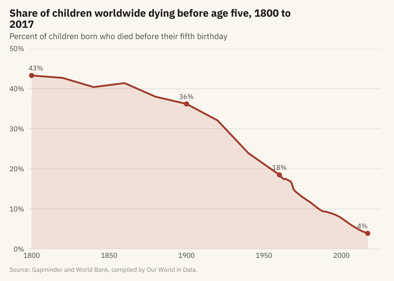
Figure 1.3
Under-five mortality rate for 191 countries, 1960 to 2017, one line per country. All but one line end lower than they start. Little else can be read from the figure, because no single line can be followed. Source: UN IGME, via Our World in Data.
Code
ggplot(u5, aes(year, under5_per_1000, group = country)) +
  geom_line(color = mv_ink$ink, alpha = 0.18, linewidth = 0.4) +
  scale_x_continuous(breaks = seq(1960, 2010, 10), expand = expansion(mult = 0.01)) +
  scale_y_continuous(expand = expansion(mult = c(0, 0.04))) +
  labs(title = "Under-five mortality in 191 countries, 1960 to 2017",
       subtitle = "Deaths before age five per 1,000 live births, one line per country",
       x = NULL, y = NULL, caption = mv_source("UN IGME, via Our World in Data")) +
  theme_mv()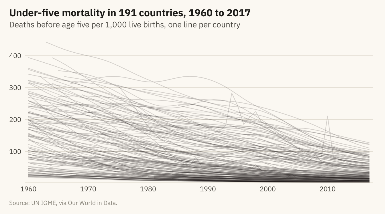
Figure 1.4
Under-five mortality by World Bank region, 1960 to 2017. The band covers the middle half of countries in each region (25th to 75th percentile) and the line is the regional median. Every region improved. South Asia started highest. Sub-Saharan Africa fell more slowly and has had the highest median since 1980. Its band is wide, so countries within the region differ as much as regions differ from each other. Source: UN IGME, via Our World in Data.
Code
region_q <- u5 |>
  group_by(region, year) |>
  summarise(lo = quantile(under5_per_1000, 0.25),
            mid = median(under5_per_1000),
            hi = quantile(under5_per_1000, 0.75), n = n(), .groups = "drop") |>
  filter(n >= 5) |>
  mutate(region = str_replace(region, " & ", " and "),
         region = fct_reorder(region, -mid, .fun = last))

ggplot(region_q, aes(year)) +
  geom_ribbon(aes(ymin = lo, ymax = hi), fill = mv_accent(), alpha = 0.18) +
  geom_line(aes(y = mid), color = mv_accent(), linewidth = 0.9) +
  facet_wrap(~ region, ncol = 3, labeller = label_wrap_gen(24)) +
  scale_x_continuous(breaks = c(1960, 1990, 2017), expand = expansion(mult = 0.02)) +
  scale_y_continuous(expand = expansion(mult = c(0, 0.04))) +
  labs(title = "Under-five mortality by region, 1960 to 2017",
       subtitle = "Deaths before age five per 1,000 births. Line: median country. Band: middle half.",
       x = NULL, y = NULL, caption = mv_source("UN IGME, via Our World in Data",
       "North America omitted (two countries)")) +
  theme_mv(base_size = 10) +
  theme(axis.text.x = element_text(size = rel(0.8)), strip.text = element_text(size = rel(0.82)))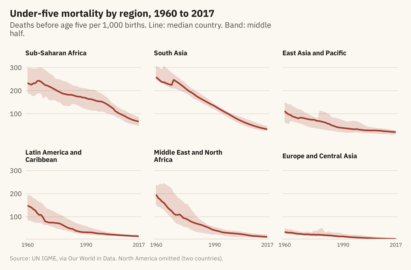
Figure 1.5
Under-five mortality in 1990 and 2017 for the twelve countries with the highest rates in 1990. Eleven of the twelve cut their rate by at least half, and Chad by 42 percent. Niger, Malawi, Liberia, and Mozambique cut theirs by more than two-thirds. Source: UN IGME, via Our World in Data.
Code
top12 <- u5 |> filter(year == 1990) |> slice_max(under5_per_1000, n = 12) |> pull(country)

slope <- u5 |>
  filter(country %in% top12, year %in% c(1990, 2017)) |>
  select(country, year, under5_per_1000) |>
  pivot_wider(names_from = year, values_from = under5_per_1000, names_prefix = "y") |>
  mutate(change = (y2017 - y1990) / y1990,
         fast = change <= -0.67) |>
  arrange(fast)  # grey rows first, so the red lines and dots draw on top

ggplot(slope) +
  geom_segment(aes(x = 1, xend = 2, y = y1990, yend = y2017, color = fast),
               linewidth = 0.8, lineend = "round") +
  geom_point(aes(x = 1, y = y1990, color = fast), size = 2) +
  geom_point(aes(x = 2, y = y2017, color = fast), size = 2) +
  geom_text_repel(aes(x = 1, y = y1990, label = paste0(country, "  ", round(y1990))),
                  hjust = 1, nudge_x = -0.08, direction = "y", size = 2.8, family = mv_font(),
                  color = mv_ink$ink2, segment.color = mv_ink$mute, segment.size = 0.3,
                  box.padding = 0.1, min.segment.length = 0) +
  geom_text_repel(aes(x = 2, y = y2017, label = paste0(round(y2017), "  ", country)),
                  hjust = 0, nudge_x = 0.08, direction = "y", size = 2.8, family = mv_font(),
                  color = mv_ink$ink2, segment.color = mv_ink$mute, segment.size = 0.3,
                  box.padding = 0.1, min.segment.length = 0) +
  scale_x_continuous(limits = c(0.4, 2.6), breaks = c(1, 2), labels = c("1990", "2017")) +
  scale_y_continuous(expand = expansion(mult = 0.05)) +
  scale_color_manual(values = c(`TRUE` = mv_accent(), `FALSE` = mv_ink$mute),
                     breaks = c("TRUE", "FALSE"),
                     labels = c("Cut by two-thirds or more", "Cut by less"), name = NULL) +
  labs(title = "Under-five mortality in 1990 and 2017, twelve highest countries in 1990",
       subtitle = "Deaths before age five per 1,000 live births",
       x = NULL, y = NULL, caption = mv_source("UN IGME, via Our World in Data")) +
  theme_mv(grid = "none") +
  theme(axis.text.y = element_blank(), legend.position = "bottom")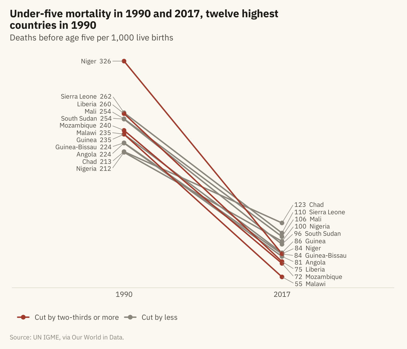
Figure 1.6
Under-five mortality in 2017, one dot per country, grouped by World Bank income classification. The lowest-income group has the highest rates and the widest spread. The medians differ by income group, and the groups overlap. Source: UN IGME, via Our World in Data; income groups from Natural Earth.
Code
now <- u5 |> filter(year == 2017) |>
  mutate(income = factor(income, levels = c("High income", "Upper middle income",
                                            "Lower middle income", "Low income")))
set.seed(11)
ggplot(now, aes(under5_per_1000, fct_rev(income))) +
  geom_jitter(height = 0.18, width = 0, size = 1.9, alpha = 0.75, color = mv_accent()) +
  stat_summary(fun = median, geom = "point", shape = 124, size = 7, color = mv_ink$ink) +
  scale_x_continuous(expand = expansion(mult = c(0.01, 0.03))) +
  labs(title = "Under-five mortality by income group, 2017",
       subtitle = "Deaths before age five per 1,000 births. One dot per country. Bar: median.",
       x = NULL, y = NULL, caption = mv_source("UN IGME, via Our World in Data")) +
  theme_mv(grid = "x")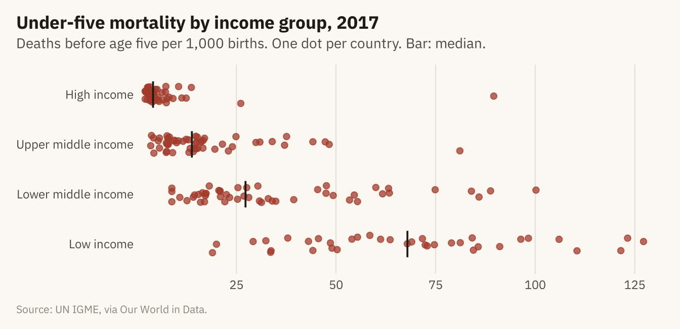
Summary statistics for the four datasets in Anscombe’s Quart
Code
anscombe_tidy <- anscombe |>
  pivot_longer(everything(), names_to = c(".value", "set"), names_pattern = "(.)(.)")

anscombe_tidy |>
  group_by(Set = set) |>
  summarise(`Mean x` = mean(x), `Mean y` = mean(y), `SD x` = sd(x), `SD y` = sd(y),
            `Correlation` = cor(x, y), .groups = "drop") |>
knitr::kable(digits = 2, align = "lrrrrr")| Set | Mean x | Mean y | SD x | SD y | Correlation |
|---|---|---|---|---|---|
| 1 | 9 | 7.5 | 3.32 | 2.03 | 0.82 |
| 2 | 9 | 7.5 | 3.32 | 2.03 | 0.82 |
| 3 | 9 | 7.5 | 3.32 | 2.03 | 0.82 |
| 4 | 9 | 7.5 | 3.32 | 2.03 | 0.82 |
Figure 1.7
Anscombe’s Quartet. The four datasets share the summary statistics in the table above and the same fitted line, drawn in each panel. Set 1 is a linear relationship with scatter. Set 2 is a curve. Set 3 is a straight line with one outlier that changes the fitted slope. Set 4 has ten points at one value of x and one point elsewhere, and that one point produces the fitted line. Source: Anscombe (1973).
Code
ggplot(anscombe_tidy, aes(x, y)) +
  geom_smooth(method = "lm", se = FALSE, color = mv_ink$mute, linewidth = 0.5, formula = y ~ x) +
  geom_point(color = mv_accent(), size = 2.2) +
  facet_wrap(~ set, ncol = 4, labeller = as_labeller(\(s) paste("Set", s))) +
  scale_x_continuous(breaks = c(5, 10, 15, 20)) +
  labs(x = NULL, y = NULL) +
  theme_mv(grid = "none") +
  theme(panel.grid.major.y = element_line(color = mv_ink$grid, linewidth = 0.3))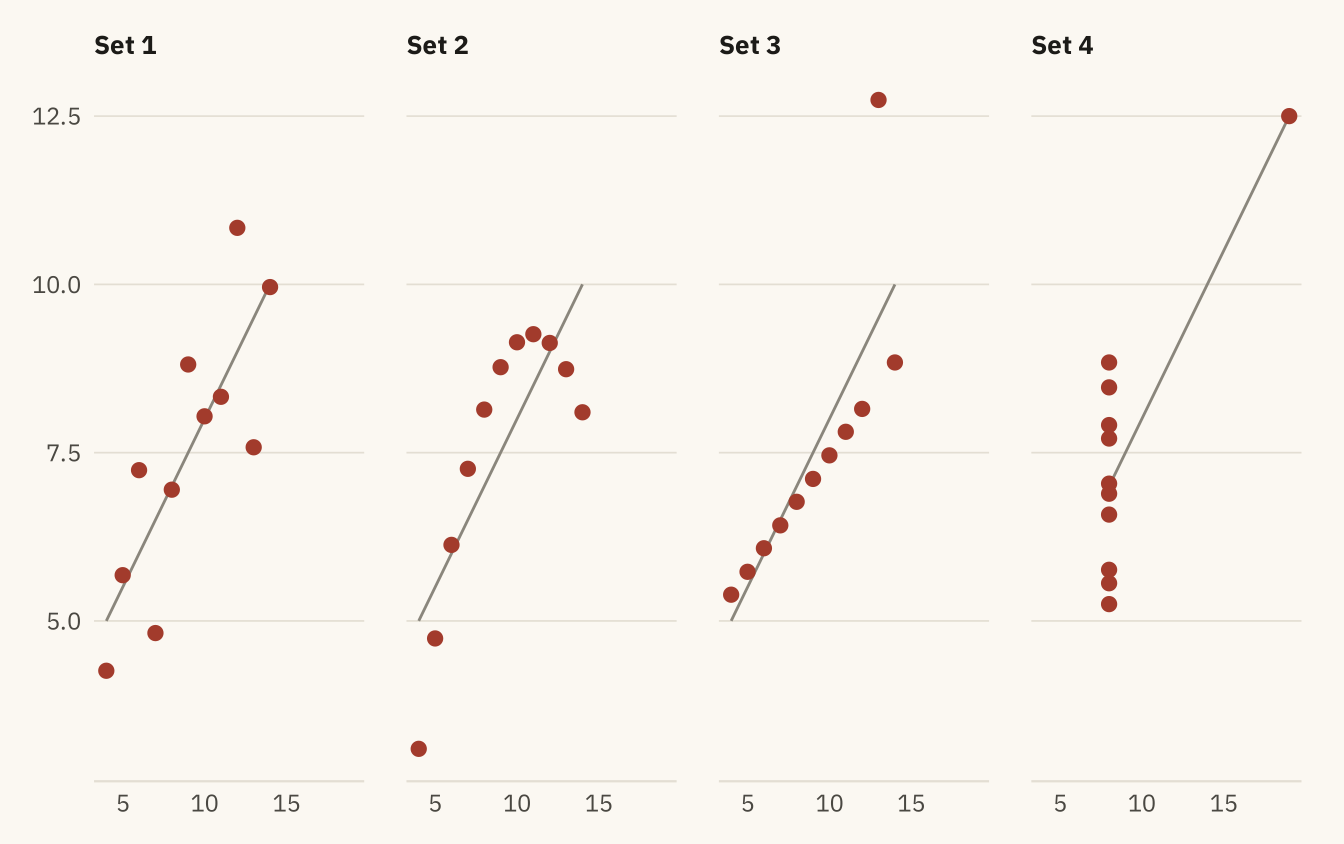
Figure 1.8
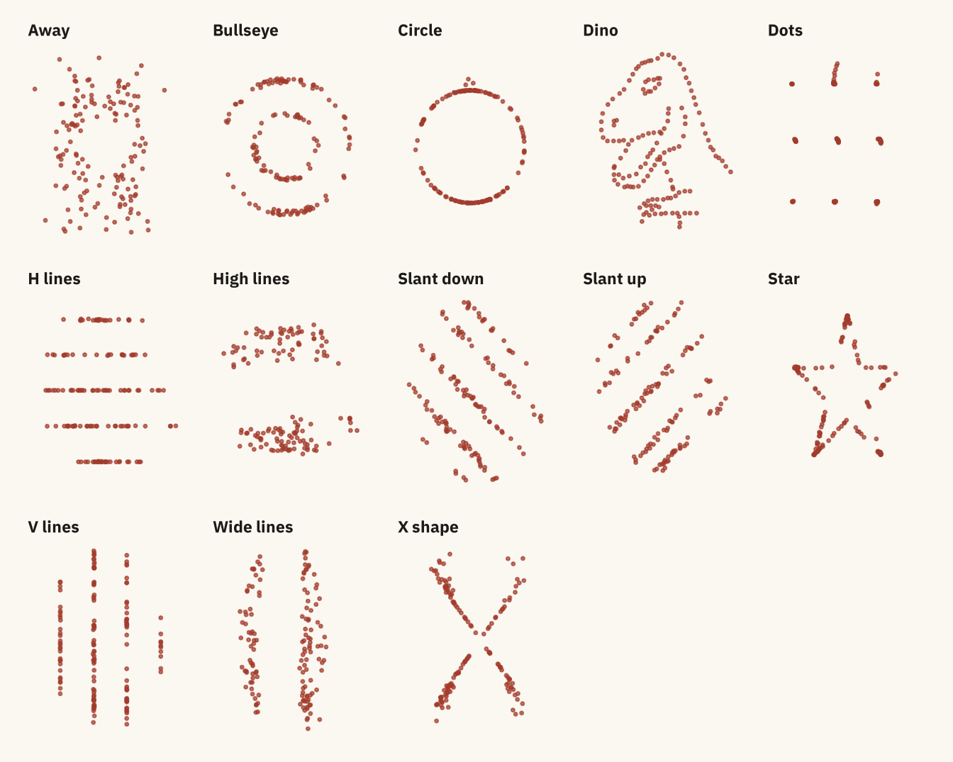
The Datasaurus Dozen. Every panel has the same mean x, mean y, standard deviation of x, standard deviation of y, and correlation, to two decimal places. Source: Matejka and Fitzmaurice (2017), via the datasauRus package.
Code
library(datasauRus)
datasaurus_dozen |>
  mutate(dataset = str_to_sentence(str_replace_all(dataset, "_", " "))) |>
  ggplot(aes(x, y)) +
  geom_point(color = mv_accent(), size = 0.55, alpha = 0.7) +
  facet_wrap(~ dataset, ncol = 5) +
  labs(x = NULL, y = NULL) +
  theme_mv(grid = "none") +
  theme(axis.text = element_blank(), axis.line.x = element_blank(),
        strip.text = element_text(size = rel(0.78)))