# Where the data and the theme live. The defaults load from the companion
# site. Set MV_DATA and MV_THEME to local paths to work offline.
mv_data  <- Sys.getenv("MV_DATA",  "https://viz.marginoferrormedia.com/data")
mv_theme <- Sys.getenv("MV_THEME", "https://viz.marginoferrormedia.com/figures/mv-theme.R")Chapter 4: Comparison and Composition
The code behind every figure in Chapter 4 of Make It Visible, in the order the chapter draws them. Run the first chunk, then any figure. Each chunk stands on its own once the setup chunk has run.
Setup
Loads the theme, the packages, and the chapter’s data.
Code
source(mv_theme)
mv_set_chapter(4)
suppressPackageStartupMessages({ library(tidyverse); library(ggrepel); library(patchwork); library(treemapify); library(ggalluvial); library(igraph); library(ggraph); library(tidygraph) })
w <- read_csv(file.path(mv_data, "ch04-refugees-world.csv"), show_col_types = FALSE) |>
  mutate(origin = str_replace(origin, " \\(.*\\)", ""), asylum = str_replace(asylum, " \\(.*\\)", ""),
         origin = recode(origin, "Syrian Arab Rep." = "Syria", "Dem. Rep. of the Congo" = "DR Congo",
                         "Central African Rep." = "Central African Rep.", "Iran" = "Iran"),
         asylum = recode(asylum, "Iran" = "Iran", "United States of America" = "United States",
                         "United Kingdom of Great Britain and Northern Ireland" = "United Kingdom",
                         "Türkiye" = "Türkiye", "Dem. Rep. of the Congo" = "DR Congo",
                         "Russian Federation" = "Russia", "United Rep. of Tanzania" = "Tanzania"))
cap_theme <- theme(plot.caption = element_text(size = 7.5, hjust = 0, color = mv_ink$mute, family = mv_font()),
                   plot.background = element_rect(fill = mv_ink$canvas, color = NA))
plain_title <- theme(plot.title = element_text(size = rel(1), face = "plain"))
src <- "UNHCR Refugee Population Statistics Database"
Figure 4.1
Refugees by country of origin at the end of 2022, ten largest. Three countries account for about three-fifths of the world’s refugees. Source: UNHCR Refugee Population Statistics Database.
Code
orig22 <- w |> filter(year == 2022) |> group_by(origin) |> summarise(r = sum(refugees), .groups = "drop")
top10 <- orig22 |> slice_max(r, n = 10) |> mutate(origin = fct_reorder(origin, r))
share3 <- sum(head(arrange(orig22, -r), 3)$r) / sum(orig22$r)

ggplot(top10, aes(r, origin)) +
  geom_col(fill = mv_accent(), width = 0.68) +
  geom_text(aes(label = label_comma(scale = 1e-6, accuracy = 0.1, suffix = " M")(r)),
            hjust = -0.15, size = 3, family = mv_font(), color = mv_ink$ink2) +
  scale_x_continuous(expand = expansion(mult = c(0, 0.15))) +
  labs(title = "Refugees by country of origin, ten largest, end of 2022",
       subtitle = "Number of refugees, in millions",
       x = NULL, y = NULL, caption = mv_source(src)) +
  theme_mv(grid = "none") +
  theme(axis.text.x = element_blank())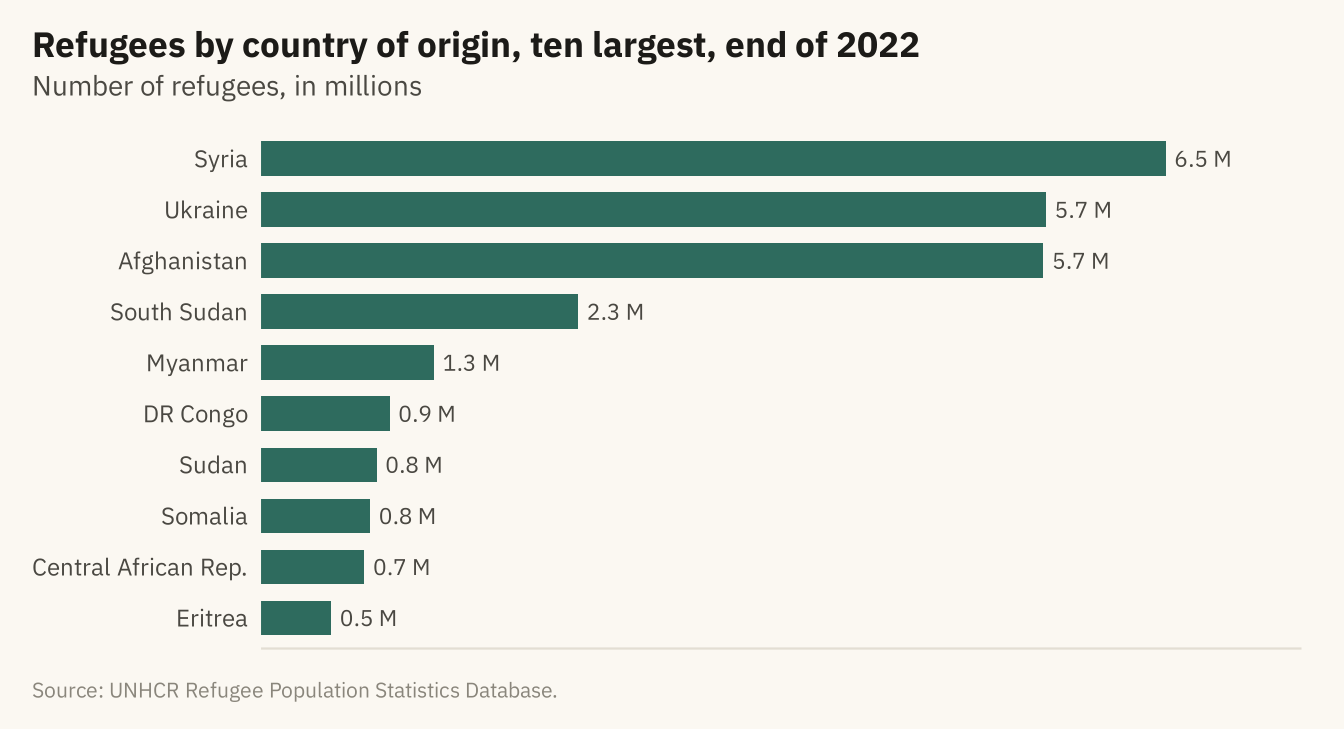
Figure 4.2
Refugees by country of origin in 2012 and 2022 for the eight largest in 2022. Left, grouped bars. The reader compares pairs of lengths. Right, a dumbbell chart. The change is drawn as a line, so the reader can compare changes across countries. Ukraine and South Sudan had few refugees in 2012. Source: UNHCR Refugee Population Statistics Database.
Code
two <- w |> filter(year %in% c(2012, 2022)) |> group_by(origin, year) |> summarise(r = sum(refugees), .groups = "drop") |>
  pivot_wider(names_from = year, values_from = r, names_prefix = "y", values_fill = 0) |>
  slice_max(y2022, n = 8) |> mutate(origin = fct_reorder(origin, y2022))

grouped <- two |> pivot_longer(c(y2012, y2022), names_to = "year", values_to = "r") |>
  mutate(year = str_remove(year, "y")) |>
  ggplot(aes(r, origin, fill = year)) +
  geom_col(position = position_dodge(width = 0.75), width = 0.7) +
  scale_fill_manual(values = c(`2012` = mv_ink$mute, `2022` = mv_accent()), name = NULL) +
  scale_x_continuous(labels = label_comma(scale = 1e-6, suffix = "M"), expand = expansion(mult = c(0, 0.05))) +
  labs(x = NULL, y = NULL, title = "Grouped bars, 2012 and 2022 values") +
  theme_mv(base_size = 10, grid = "x") + plain_title

dumbbell <- ggplot(two) +
  geom_segment(aes(x = y2012, xend = y2022, y = origin, yend = origin), color = mv_ink$grid, linewidth = 1.6) +
  geom_point(aes(y2012, origin), color = mv_ink$mute, size = 2.6) +
  geom_point(aes(y2022, origin), color = mv_accent(), size = 2.6) +
  annotate("text", x = two$y2012[two$origin == "Ukraine"], y = "Ukraine", label = "2012", vjust = -1.1,
           size = 2.8, family = mv_font(), color = mv_ink$mute) +
  annotate("text", x = two$y2022[two$origin == "Ukraine"], y = "Ukraine", label = "2022", vjust = -1.1,
           size = 2.8, family = mv_font(), color = mv_accent()) +
  scale_x_continuous(labels = label_comma(scale = 1e-6, suffix = "M"), expand = expansion(mult = c(0.02, 0.08))) +
  labs(x = NULL, y = NULL, title = "Dumbbell, change from 2012 to 2022") +
  theme_mv(base_size = 10, grid = "x") + plain_title

grouped + dumbbell + plot_annotation(caption = mv_source(src), theme = cap_theme)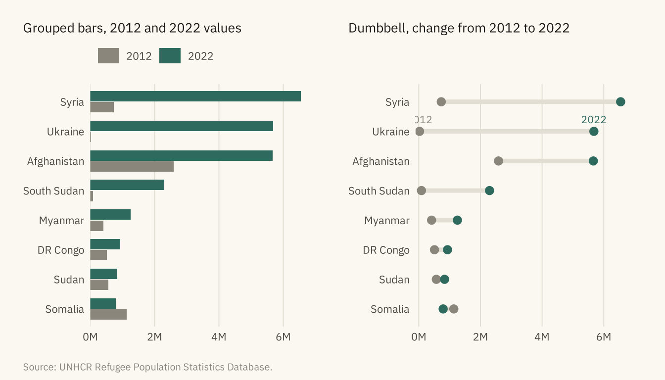
Figure 4.3
Where the refugees from the five largest countries of origin were hosted at the end of 2022, as shares. In each row the darkest segment is the single largest host country, named on the bar. For four of the five, the largest host was a neighboring country. Source: UNHCR Refugee Population Statistics Database.
Code
five <- head(arrange(orig22, -r), 5)$origin
comp <- w |> filter(year == 2022, origin %in% five) |>
  group_by(origin, asylum) |> summarise(r = sum(refugees), .groups = "drop") |>
  group_by(origin) |> arrange(-r, .by_group = TRUE) |>
  mutate(rank = row_number(), host = case_when(rank == 1 ~ asylum, rank == 2 ~ asylum, rank == 3 ~ asylum, TRUE ~ "All others"),
         slot = case_when(rank == 1 ~ "Largest host", rank == 2 ~ "Second", rank == 3 ~ "Third", TRUE ~ "All others")) |>
  group_by(origin, slot, host) |> summarise(r = sum(r), .groups = "drop") |>
  group_by(origin) |> mutate(share = r / sum(r), total = sum(r)) |> ungroup() |>
  mutate(slot = factor(slot, levels = rev(c("Largest host", "Second", "Third", "All others"))),
         origin = fct_reorder(origin, total),
         label = if_else(slot == "Largest host", paste0(host, "  ", percent(share, 1)), ""))

ggplot(comp, aes(share, origin, fill = slot)) +
  geom_col(width = 0.7, color = mv_ink$canvas, linewidth = 0.4) +
  geom_text(aes(label = label, x = 0.01), position = position_stack(vjust = 0, reverse = FALSE),
            hjust = 0, size = 3, family = mv_font(), color = mv_ink$canvas, fontface = "bold") +
  scale_fill_manual(values = c(`Largest host` = mv_accent(), Second = "#5E9484", Third = "#A9C7BC", `All others` = mv_ink$grid),
                    breaks = c("Largest host", "Second", "Third", "All others"), name = NULL) +
  scale_x_continuous(labels = label_percent(), expand = expansion(0)) +
  labs(title = "Share of each origin's refugees by host country, end of 2022",
       subtitle = "Percent of refugees from each of the five largest origins. Largest host named on each bar.",
       x = NULL, y = NULL, caption = mv_source(src)) +
  theme_mv(grid = "none") +
  theme(legend.position = "bottom", axis.text.x = element_blank())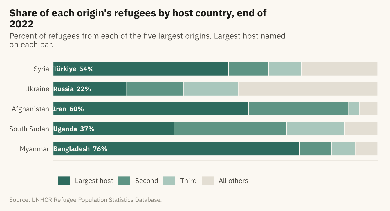
Figure 4.4
Share of the world’s refugees hosted by countries in each World Bank income group, end of 2022. Three in four are in low- and middle-income countries. A pie is suitable here because the reader only needs to see that the high-income slice is about a quarter. Source: UNHCR; income groups from Natural Earth.
Code
inc <- w |> filter(year == 2022, !is.na(asylum_income)) |>
  mutate(grp = if_else(asylum_income == "High income", "High income", "Low and middle income")) |>
  group_by(grp) |> summarise(r = sum(refugees), .groups = "drop") |> mutate(share = r / sum(r))

ggplot(inc, aes(x = 1, y = share, fill = grp)) +
  geom_col(width = 1, color = mv_ink$canvas, linewidth = 0.8) +
  coord_polar(theta = "y", start = 0) +
  geom_text(aes(label = percent(share, 1)), position = position_stack(vjust = 0.5), size = 4.2,
            family = mv_font(), color = mv_ink$canvas, fontface = "bold") +
  scale_fill_manual(values = c(`High income` = mv_ink$mute, `Low and middle income` = mv_accent()), name = NULL) +
  labs(title = "Share of refugees by income group\nof host country, end of 2022",
       caption = mv_source("UNHCR; Natural Earth income groups")) +
  theme_mv_blank() + theme(legend.position = "bottom", plot.title = element_text(hjust = 0.5, lineheight = 1.05))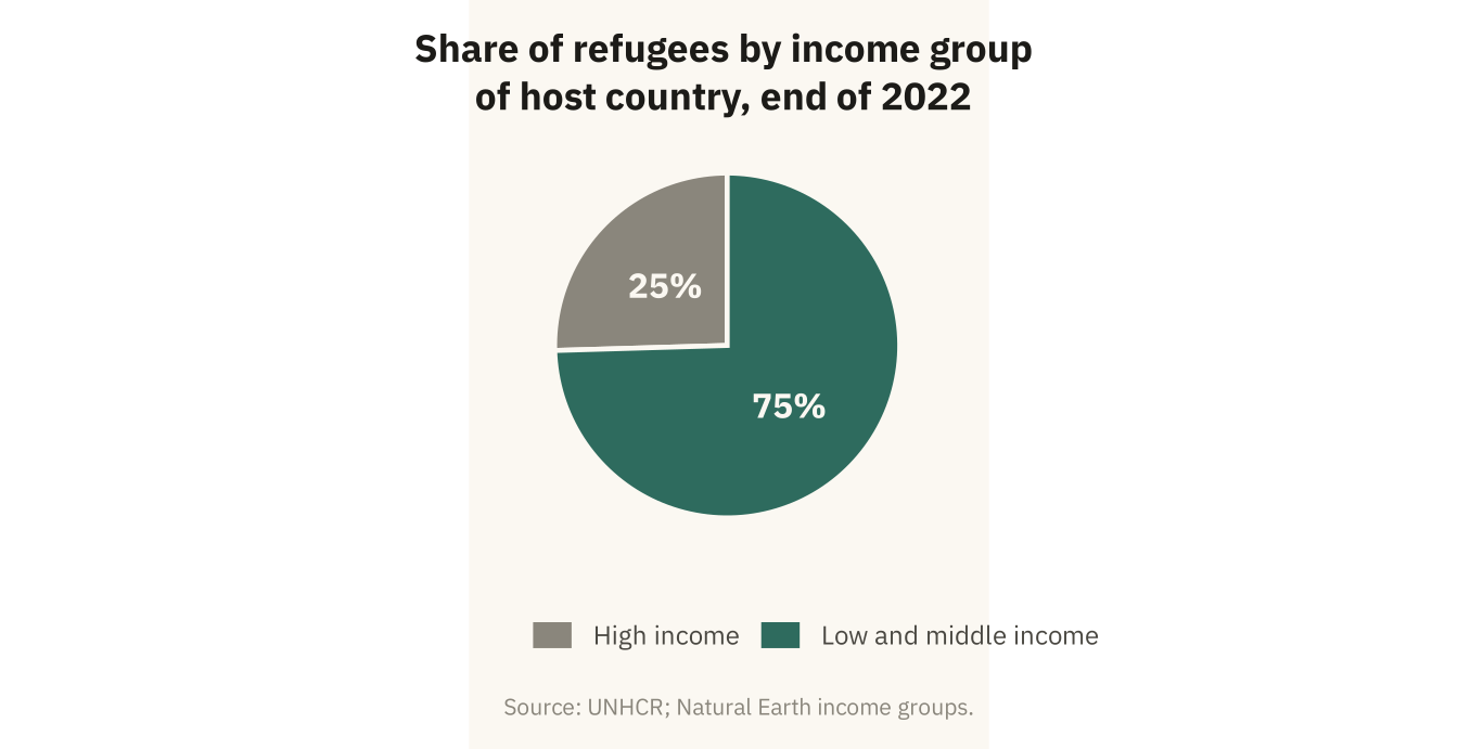
Figure 4.5
The thirty countries hosting the most refugees at the end of 2022. Position encodes the count. Color groups the countries by World Bank region. Source: UNHCR; regions from Natural Earth.
Code
hosts30 <- w |> filter(year == 2022, !is.na(asylum_region)) |>
  group_by(asylum, asylum_region) |> summarise(r = sum(refugees), .groups = "drop") |>
  slice_max(r, n = 30) |>
  mutate(asylum = fct_reorder(asylum, r),
         asylum_region = str_replace(asylum_region, " & ", " and "))
reg_cols <- c("Sub-Saharan Africa" = mv_accent(), "Middle East and North Africa" = "#B8862B",
              "Europe and Central Asia" = "#1C1B18", "South Asia" = "#7A4E8C",
              "East Asia and Pacific" = "#5B6E8C", "Latin America and Caribbean" = "#C25B2A",
              "North America" = "#8A867C")
ggplot(hosts30, aes(r, asylum, color = asylum_region)) +
  geom_segment(aes(x = 0, xend = r, yend = asylum), color = mv_ink$grid, linewidth = 0.5) +
  geom_point(size = 2.6) +
  scale_color_manual(values = reg_cols, name = NULL) +
  scale_x_continuous(labels = label_comma(scale = 1e-6, suffix = "M"), expand = expansion(mult = c(0, 0.04))) +
  guides(color = guide_legend(ncol = 2)) +
  labs(title = "Refugees hosted, thirty largest host countries, end of 2022",
       subtitle = "Number of refugees, in millions. Color: World Bank region.",
       x = NULL, y = NULL, caption = mv_source("UNHCR; Natural Earth regions")) +
  theme_mv(base_size = 10, grid = "x") +
  theme(legend.text = element_text(size = rel(0.78)), axis.text.y = element_text(size = rel(0.85)))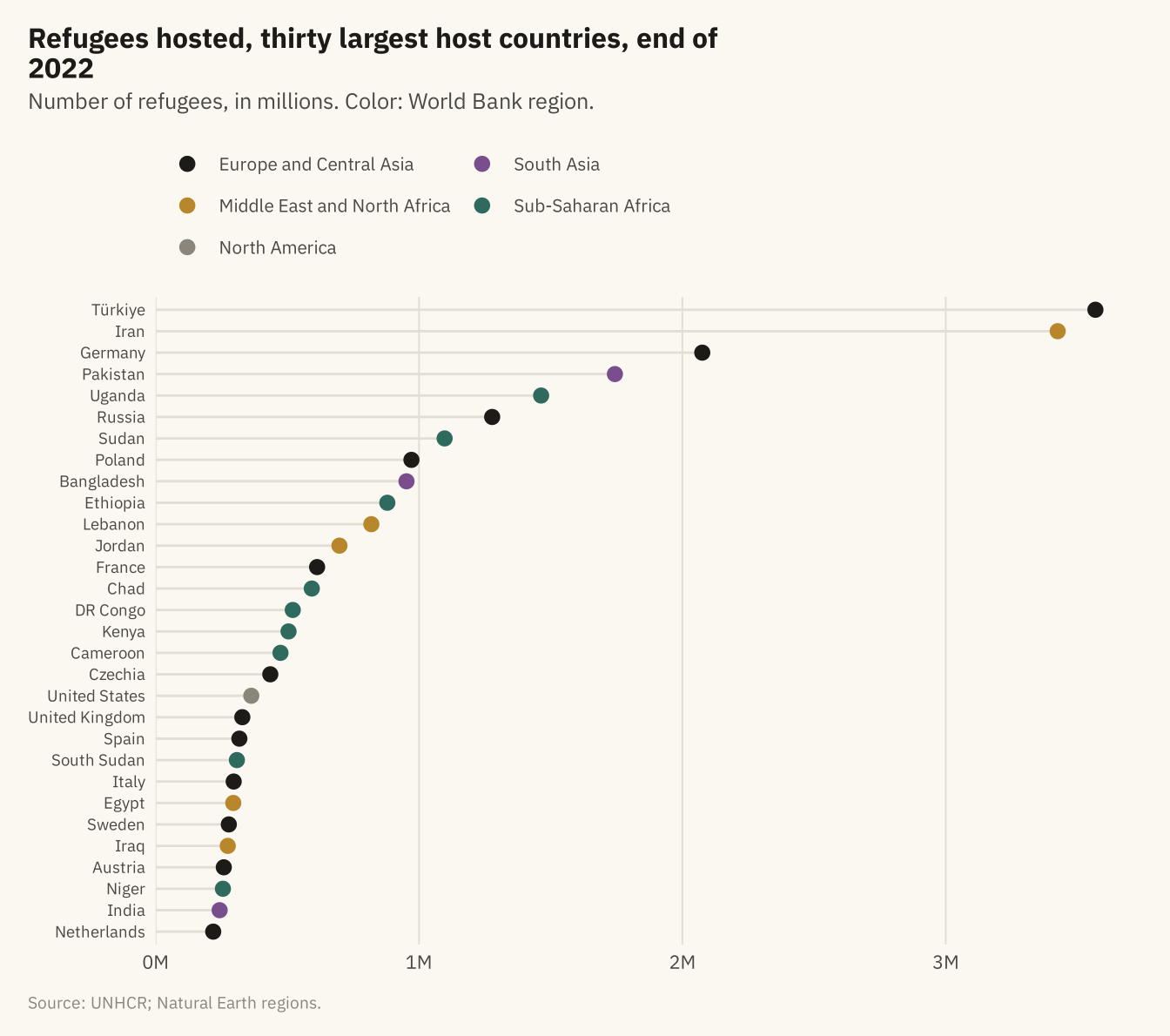
Figure 4.6
All refugees at the end of 2022 by host region and host country. Each rectangle is a host country, sized by the number of refugees and grouped by region. Countries hosting fewer than 200,000 are unlabeled. The three smallest regions, North America, East Asia and Pacific, and Latin America and Caribbean, are too small to name on the chart. Source: UNHCR; regions from Natural Earth.
Code
tm <- w |> filter(year == 2022, !is.na(asylum_region)) |>
  group_by(asylum_region, asylum) |> summarise(r = sum(refugees), .groups = "drop") |>
  mutate(asylum_region = str_replace(asylum_region, " & ", " and "),
         lab = if_else(r >= 200000, asylum, ""),
         # Small regions get a blank subgroup name so no label is drawn over their tiles.
         # Distinct whitespace strings keep each region as its own subgroup in the layout.
         region_lab = case_when(asylum_region == "North America" ~ " ",
                                asylum_region == "East Asia and Pacific" ~ "  ",
                                asylum_region == "Latin America and Caribbean" ~ "   ",
                                TRUE ~ asylum_region))
ggplot(tm, aes(area = r, fill = asylum_region, subgroup = region_lab, label = lab)) +
  geom_treemap(color = mv_ink$canvas, size = 1.5) +
  geom_treemap_subgroup_border(color = mv_ink$canvas, size = 4) +
  geom_treemap_text(color = mv_ink$canvas, family = mv_font(), size = 9, min.size = 4,
                    padding.x = grid::unit(1, "mm"), padding.y = grid::unit(1.5, "mm"), reflow = TRUE) +
  geom_treemap_subgroup_text(color = mv_ink$canvas, family = mv_font(), fontface = "bold", alpha = 0.55,
                             size = 14, place = "bottomright", grow = FALSE, reflow = TRUE) +
  scale_fill_manual(values = reg_cols, guide = "none") +
  labs(title = "Refugees by host country and region, end of 2022",
       subtitle = "Each rectangle is a host country, sized by refugees hosted. 29 million refugees in total.",
       caption = mv_source("UNHCR; Natural Earth regions")) +
  theme_mv_blank()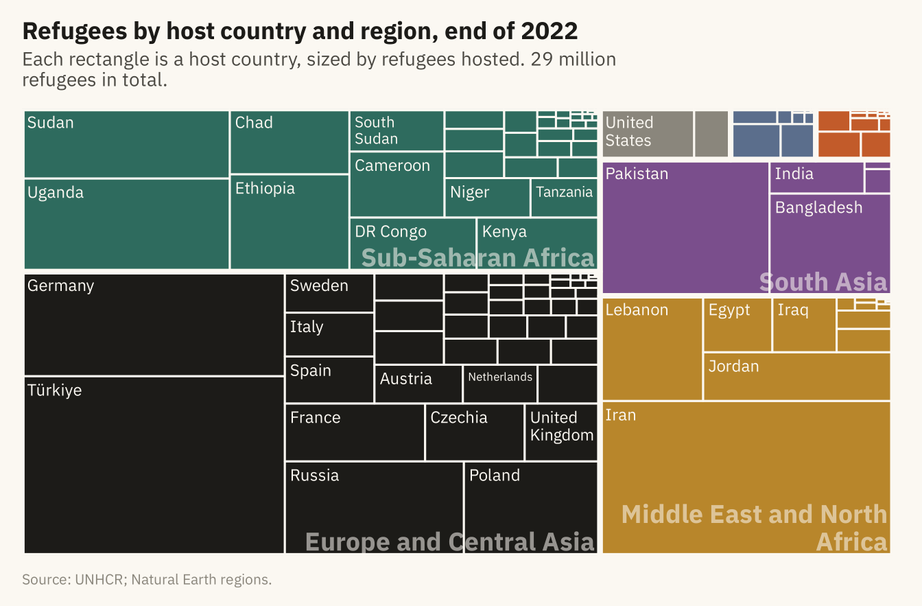
Figure 4.7
The three largest countries of origin for refugees hosted in each World Bank region, end of 2022. Each panel is sorted on its own, and the panels share one horizontal scale so sizes can be compared across regions. Source: UNHCR; regions from Natural Earth.
Code
by_reg <- w |> filter(year == 2022, !is.na(asylum_region), asylum_region != "North America") |>
  group_by(asylum_region, origin) |> summarise(r = sum(refugees), .groups = "drop") |>
  group_by(asylum_region) |> slice_max(r, n = 3) |> ungroup() |>
  mutate(asylum_region = str_replace(asylum_region, " & ", " and "),
         asylum_region = str_wrap(asylum_region, 14),
         asylum_region = fct_reorder(asylum_region, r, .fun = max, .desc = TRUE),
         origin = paste0(origin, "___", as.integer(asylum_region)))
by_reg <- by_reg |> mutate(origin = fct_reorder(origin, r))
ggplot(by_reg, aes(r, origin)) +
  geom_col(fill = mv_accent(), width = 0.7) +
  facet_wrap(~ asylum_region, ncol = 3, scales = "free_y") +
  scale_y_discrete(labels = \(x) str_remove(x, "___\\d+$")) +
  scale_x_continuous(labels = label_comma(scale = 1e-6, suffix = "M"), breaks = c(0, 3e6, 6e6),
                     expand = expansion(mult = c(0, 0.05))) +
  labs(title = "Three largest countries of origin by host region, end of 2022",
       subtitle = "Number of refugees, in millions. Panels share one horizontal scale.",
       x = NULL, y = NULL, caption = mv_source("UNHCR; Natural Earth regions")) +
  theme_mv(base_size = 10, grid = "x") +
  theme(strip.text = element_text(size = rel(0.8), lineheight = 0.95))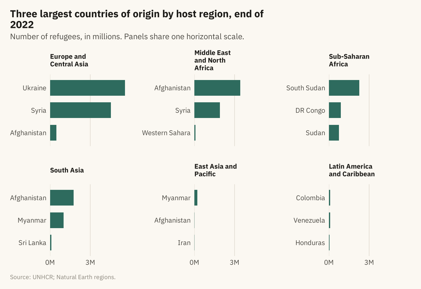
Figure 4.8
The twelve largest refugee flows from country of origin to country of asylum at the end of 2022. The width of each band is proportional to the number of refugees. The five origins on the left and the eleven hosts on the right are sorted by size. Together these twelve flows hold about 56 percent of the world’s 29.4 million refugees. Source: UNHCR.
Code
flows <- w |> filter(year == 2022) |>
  group_by(origin, asylum) |> summarise(n = sum(refugees), .groups = "drop") |>
  slice_max(n, n = 12) |>
  mutate(origin = fct_reorder(origin, n, .fun = sum, .desc = TRUE),
         asylum = fct_reorder(asylum, n, .fun = sum, .desc = TRUE))
ggplot(flows, aes(axis1 = origin, axis2 = asylum, y = n)) +
  geom_alluvium(aes(fill = origin), width = 0.18, alpha = 0.75, knot.pos = 0.4) +
  geom_stratum(width = 0.18, fill = mv_ink$canvas, color = mv_ink$ink2, linewidth = 0.4) +
  geom_text(stat = "stratum", aes(label = after_stat(stratum)), size = 2.7, family = mv_font(), color = mv_ink$ink) +
  scale_x_discrete(limits = c("Origin", "Asylum"), expand = expansion(mult = 0.25)) +
  scale_fill_manual(values = mv_series(6), guide = "none") +
  scale_y_continuous(labels = label_comma(scale = 1e-6, suffix = "M"), expand = expansion(0)) +
  labs(title = "The twelve largest refugee flows, end of 2022",
       subtitle = "From country of origin to country of asylum. Band width is the number of refugees, in millions.",
       x = NULL, y = NULL, caption = mv_source(src)) +
  theme_mv(grid = "none") + theme(axis.text.y = element_blank())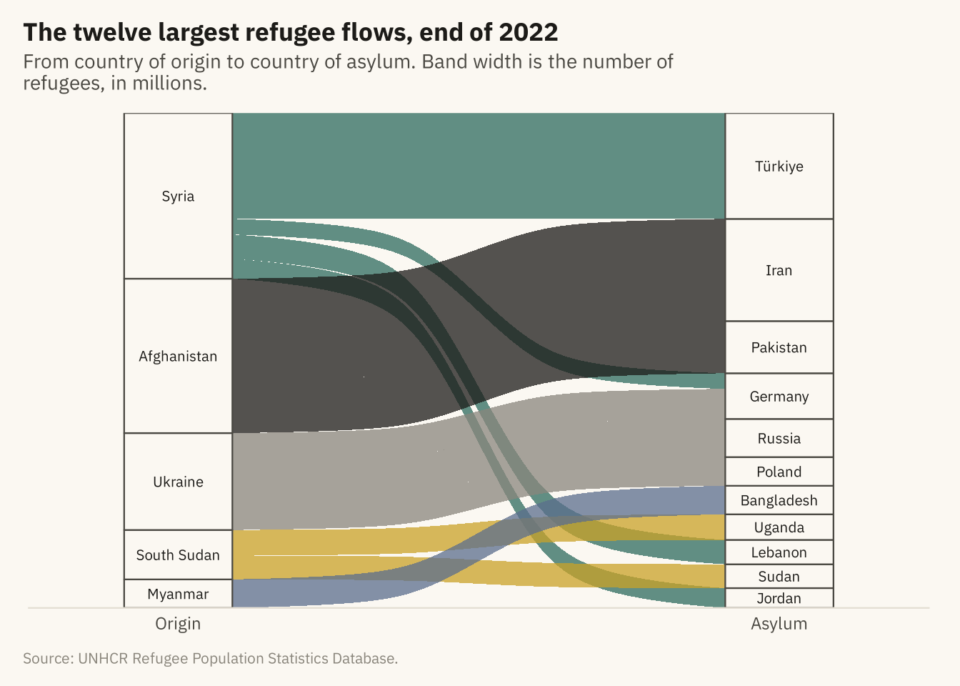
Figure 4.9
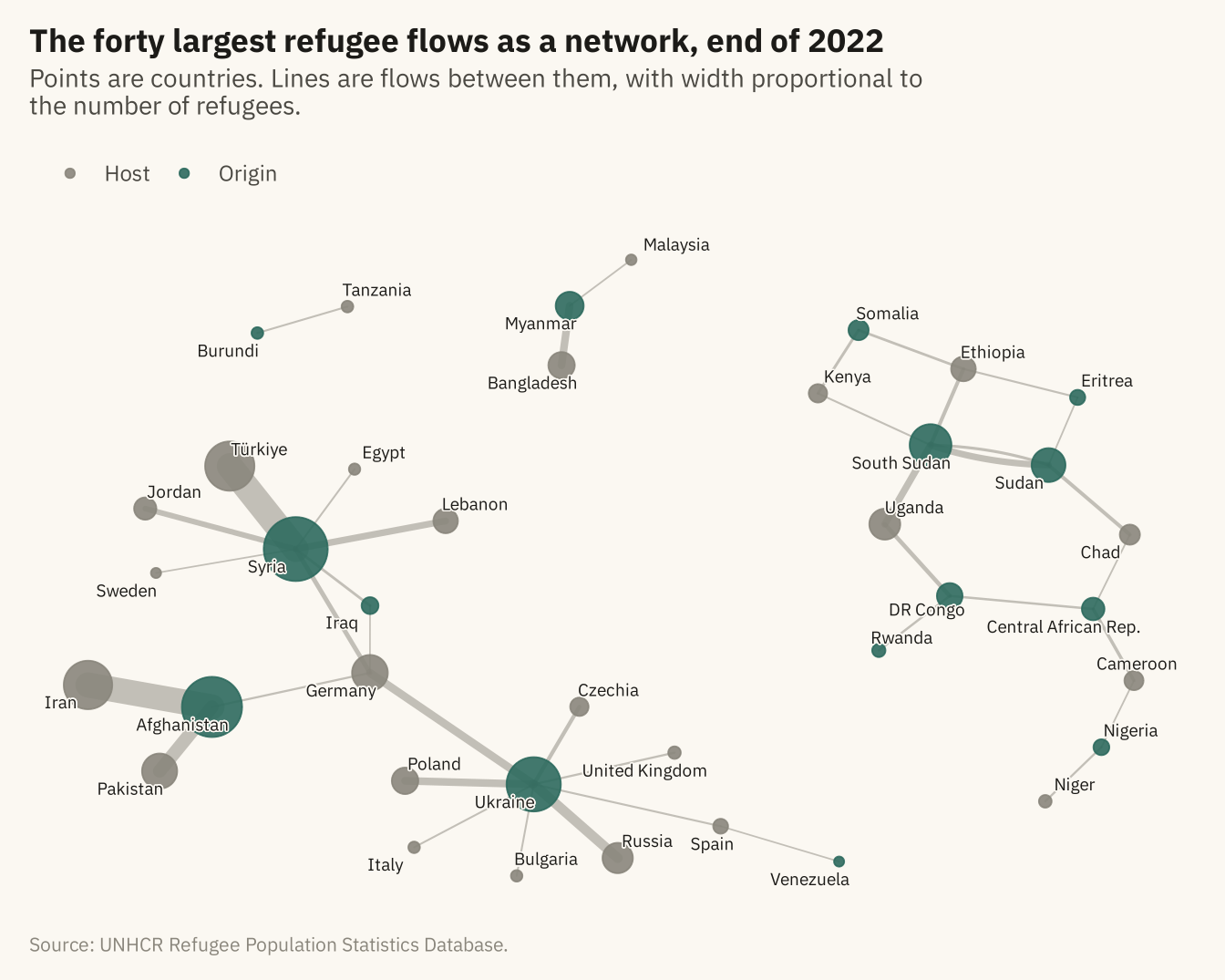
The forty largest refugee flows at the end of 2022 drawn as a network. Each point is a country, sized by the total number of refugees it sent or hosted among these flows. Each line is a flow, with width proportional to its size. Origins are in color and hosts in grey. Countries that are both, such as Sudan and DR Congo, are colored as origins. Source: UNHCR.
Code
edges <- w |> filter(year == 2022) |>
  group_by(origin, asylum) |> summarise(n = sum(refugees), .groups = "drop") |>
  slice_max(n, n = 40) |> rename(from = origin, to = asylum, weight = n)
g <- as_tbl_graph(edges, directed = TRUE) |>
  mutate(total = centrality_degree(weights = weight, mode = "all"),
         role = if_else(name %in% edges$from, "Origin", "Host"))
set.seed(4)
ggraph(g, layout = "fr", weights = NA, niter = 2000) +
  geom_edge_fan(aes(width = weight), color = mv_ink$mute, alpha = 0.5, lineend = "round") +
  geom_node_point(aes(size = total, color = role), alpha = 0.9) +
  geom_node_text(aes(label = name), size = 2.5, family = mv_font(), color = mv_ink$ink, repel = TRUE,
                 max.overlaps = 30, bg.color = mv_ink$canvas, bg.r = 0.12) +
  scale_edge_width(range = c(0.3, 5), guide = "none") +
  scale_size_area(max_size = 12, guide = "none") +
  scale_color_manual(values = c(Origin = mv_accent(), Host = mv_ink$mute), name = NULL) +
  labs(title = "The forty largest refugee flows as a network, end of 2022",
       subtitle = "Points are countries. Lines are flows between them, with width proportional to the number of refugees.",
       caption = mv_source(src)) +
  theme_mv_blank() +
  theme(panel.grid = element_blank(), legend.position = "top")