# Where the data and the theme live. The defaults load from the companion
# site. Set MV_DATA and MV_THEME to local paths to work offline.
mv_data  <- Sys.getenv("MV_DATA",  "https://viz.marginoferrormedia.com/data")
mv_theme <- Sys.getenv("MV_THEME", "https://viz.marginoferrormedia.com/figures/mv-theme.R")Chapter 11: Interactivity and Dashboards
The code behind every figure in Chapter 11 of Make It Visible, in the order the chapter draws them. Run the first chunk, then any figure. Each chunk stands on its own once the setup chunk has run.
Setup
Loads the theme, the packages, and the chapter’s data.
Code
source(mv_theme)
mv_set_chapter(11)
suppressPackageStartupMessages({ library(tidyverse); library(ggrepel); library(patchwork); library(sf) })
sf_use_s2(FALSE)
gaps <- read_csv(file.path(mv_data, "ch11-zip-gaps.csv"), show_col_types = FALSE)
orgs <- read_csv(file.path(mv_data, "ch11-orgs.csv"), show_col_types = FALSE)
cs   <- read_csv(file.path(mv_data, "ch11-county-summary.csv"), show_col_types = FALSE)
co   <- st_read(file.path(mv_data, "ch08-counties.geojson"), quiet = TRUE)
inw  <- co |> filter(fips %in% as.character(cs$fips))
cap_theme <- theme(plot.caption = element_text(size = 7.5, hjust = 0, color = mv_ink$mute, family = mv_font()),
                   plot.background = element_rect(fill = mv_ink$canvas, color = NA))
plain_title <- theme(plot.title = element_text(size = rel(1), face = "plain"))
src <- "Inland Northwest Nonprofit Sector Intelligence (NCCS, IRS Form 990, ACS 2019 to 2023)"
g2 <- gaps |> filter(population >= 500) |> mutate(county = str_remove(county, " County"))
g2 <- g2 |> mutate(gap = poverty_rate > median(poverty_rate) & hs_per_1k < median(hs_per_1k))
n_gap <- sum(g2$gap)
Figure 11.1
ZIP codes in the seven-county Inland Northwest with at least 500 residents, by poverty rate and human-services nonprofits per 1,000 residents, sized by population. Downtown Spokane (99201) has the most organizations per resident and the highest poverty rate of any large ZIP. One small ZIP in Stevens County (99126) has a higher poverty rate and no organizations. The ZIPs in the lower right have high poverty and few organizations. Source: Inland Northwest Nonprofit Sector Intelligence (NCCS, IRS Form 990, ACS 2019 to 2023).
Code
named <- g2 |> filter(zip %in% c("99201", "99207", "99163", "99001", "99004", "99202", "83843", "99016", "99212"))
ggplot(g2, aes(poverty_rate, hs_per_1k)) +
  geom_hline(yintercept = median(g2$hs_per_1k), color = mv_ink$grid, linewidth = 0.5) +
  geom_vline(xintercept = median(g2$poverty_rate), color = mv_ink$grid, linewidth = 0.5) +
  geom_point(aes(size = population), color = mv_accent(), alpha = 0.5) +
  geom_point(data = named, aes(size = population), color = mv_ink$ink, shape = 21, stroke = 0.5, fill = NA) +
  geom_text_repel(data = named, aes(label = paste0(zip, " ", county)), size = 2.6, family = mv_font(), color = mv_ink$ink,
                  min.segment.length = 0, segment.color = mv_ink$mute, segment.size = 0.3, box.padding = 0.5, seed = 4) +
  annotate("text", x = 33.5, y = 1.6, label = "High poverty,\nfew services", hjust = 1, vjust = 0, size = 3, family = mv_font(), color = mv_ink$ink2, lineheight = 0.95, fontface = "bold") +
  scale_size_area(max_size = 12, guide = "none") +
  scale_x_continuous(labels = label_percent(scale = 1)) +
  scale_y_continuous(expand = expansion(mult = c(0.02, 0.08))) +
  labs(title = "Poverty rate and human-services nonprofits per 1,000 residents, by ZIP code",
       subtitle = "Seven Inland Northwest counties, ZIPs with 500 or more residents, sized by population",
       x = "Poverty rate", y = "Human-services nonprofits per 1,000 residents",
       caption = mv_source(src)) +
  theme_mv(grid = "y") + theme(panel.grid.major.x = element_line(color = mv_ink$grid, linewidth = 0.35))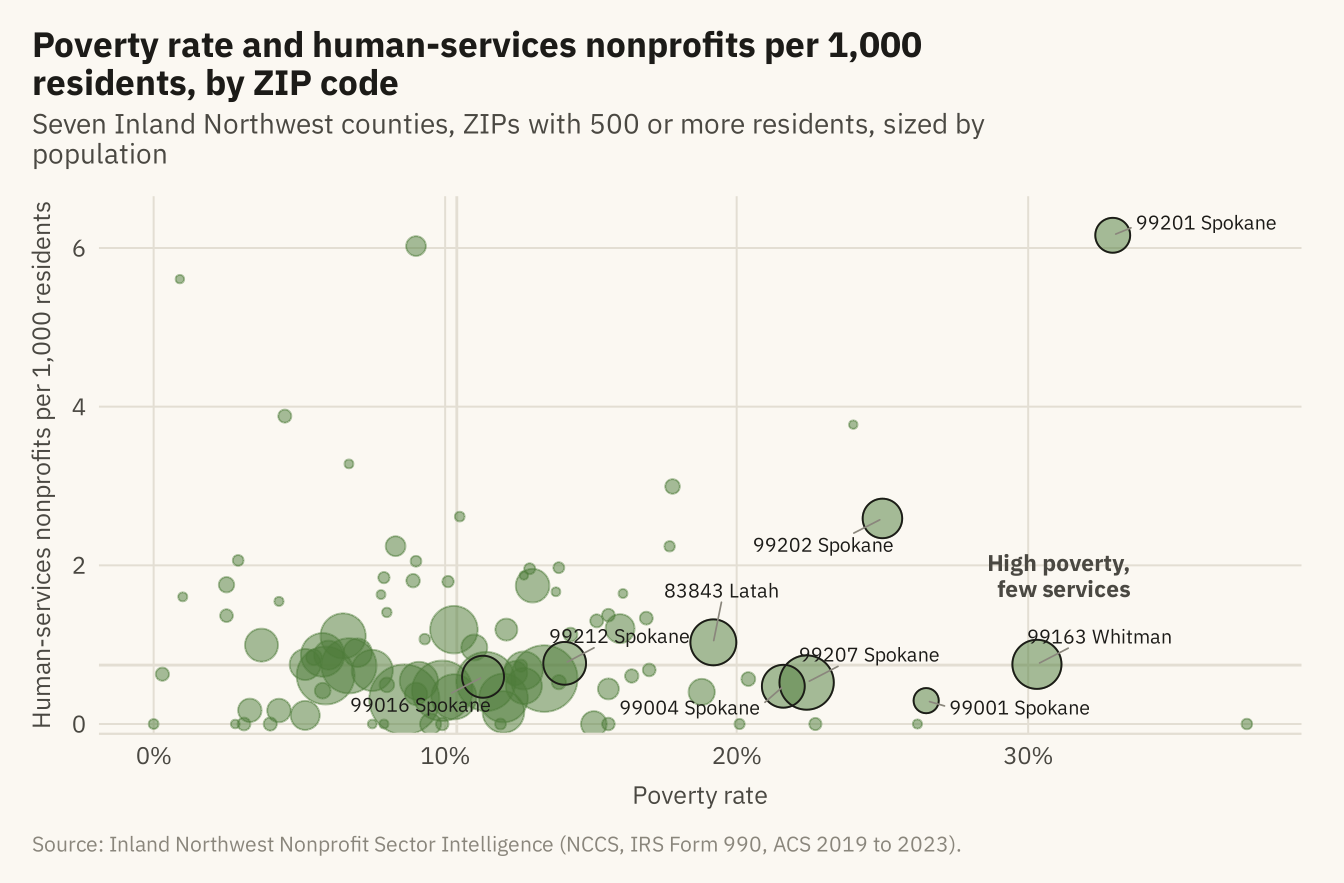
Figure 11.2
The same chart with details on demand. Online, hovering over any point shows the ZIP code, county, population, poverty rate, and number of human-services organizations. The labels from the previous figure have been removed, because the reader can now ask for any of them. Source: Inland Northwest Nonprofit Sector Intelligence.
Code
p <- ggplot(g2, aes(poverty_rate, hs_per_1k,
                    text = paste0("ZIP ", zip, ", ", county, " County\nPopulation ", label_comma()(population),
                                  "\nPoverty rate ", poverty_rate, "%\n", n_human_services, " human-services organizations"))) +
  geom_hline(yintercept = median(g2$hs_per_1k), color = mv_ink$grid, linewidth = 0.5) +
  geom_vline(xintercept = median(g2$poverty_rate), color = mv_ink$grid, linewidth = 0.5) +
  geom_point(aes(size = population), color = mv_accent(), alpha = 0.55) +
  scale_size_area(max_size = 12, guide = "none") +
  scale_x_continuous(labels = label_percent(scale = 1)) +
  labs(title = "Poverty rate and human-services nonprofits per 1,000 residents, by ZIP code", x = "Poverty rate", y = "Human-services nonprofits per 1,000 residents") +
  theme_mv(grid = "y") + theme(panel.grid.major.x = element_line(color = mv_ink$grid, linewidth = 0.35))
if (knitr::is_html_output(excludes = "epub")) {
  plotly::ggplotly(p, tooltip = "text") |>
    plotly::config(displayModeBar = FALSE) |>
    plotly::layout(font = list(family = "IBM Plex Sans, Inter, sans-serif"),
                   paper_bgcolor = mv_ink$canvas, plot_bgcolor = mv_ink$canvas)
} else {
  p + labs(subtitle = "Interactive in the online edition at viz.marginoferrormedia.com", caption = mv_source(src))
}
Figure 11.3
The overview chart split by county, with all ZIPs in grey behind each panel. Spokane County has the most ZIPs, 33 of 94. The ZIPs with the highest coverage are small towns in Whitman, Latah, and Stevens, plus downtown Spokane. The one large point in Whitman County is Pullman, a university town with a high student poverty rate. Source: Inland Northwest Nonprofit Sector Intelligence.
Code
ggplot(g2, aes(poverty_rate, hs_per_1k)) +
  geom_point(data = select(g2, -county), color = mv_ink$grid, size = 0.9) +
  geom_point(aes(size = population), color = mv_accent(), alpha = 0.6) +
  facet_wrap(~ county, ncol = 4) +
  scale_size_area(max_size = 8, guide = "none") +
  scale_x_continuous(labels = label_percent(scale = 1), breaks = c(0, 15, 30)) +
  labs(title = "Poverty rate and human-services nonprofits per 1,000 residents, by county",
       subtitle = "Each panel shows one county in color, with every ZIP in grey",
       x = "Poverty rate", y = "Human-services nonprofits per 1,000", caption = mv_source(src)) +
  theme_mv(base_size = 10) + theme(strip.text = element_text(size = rel(0.85)))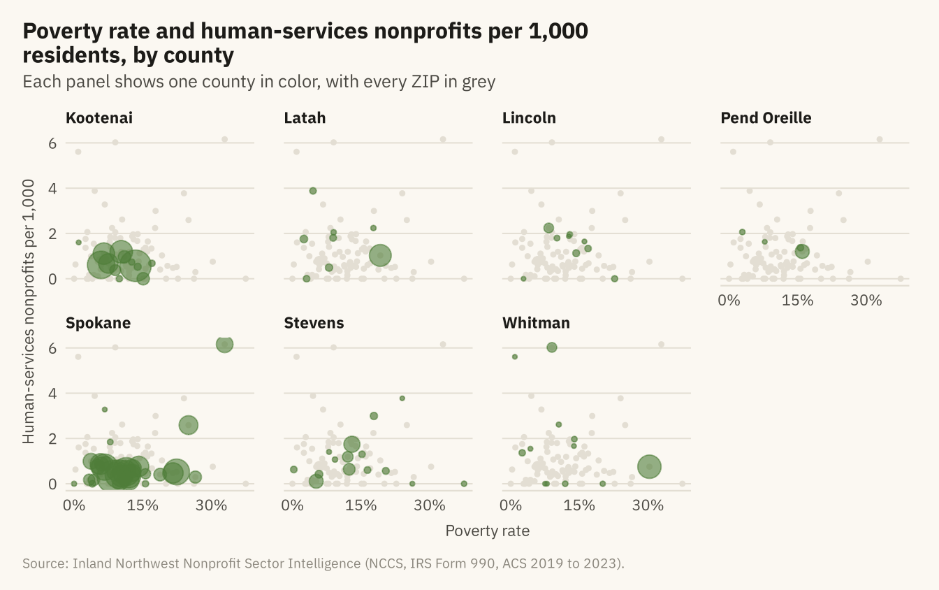
Figure 11.4
ZIP codes over the seven counties, sized by population and colored by whether they fall in the high-poverty, low-coverage quadrant of the overview chart. Twelve of the 25 dark points are in Spokane County, most of them in the Valley and on the north side. Five are in Kootenai County and eight are in the rural counties. Source: Inland Northwest Nonprofit Sector Intelligence; county boundaries from the US Census Bureau.
Code
cty_lab <- tribble(~county, ~lon, ~lat,
  "Kootenai", -116.42, 47.42, "Latah", -116.71, 46.93, "Lincoln", -118.42, 47.70,
  "Pend Oreille", -117.27, 48.65, "Spokane", -117.62, 47.30, "Stevens", -118.02, 48.18, "Whitman", -117.52, 47.02)
ggplot() +
  geom_sf(data = inw, fill = "#F2EDE2", color = mv_ink$canvas, linewidth = 0.6) +
  geom_point(data = g2, aes(lon, lat, size = population, color = gap), alpha = 0.7) +
  geom_label(data = cty_lab, aes(lon, lat, label = county), size = 2.6, family = mv_font(), color = mv_ink$ink2,
             fill = alpha(mv_ink$canvas, 0.75), label.size = 0, label.padding = unit(0.12, "lines")) +
  scale_color_manual(values = c(`TRUE` = mv_ink$ink, `FALSE` = mv_accent()), labels = c("Other ZIPs", "High poverty, few services"), name = NULL) +
  scale_size_area(max_size = 10, guide = "none") +
  coord_sf(default_crs = 4326) +
  labs(title = "ZIP codes with high poverty and\nfew human-services nonprofits",
       subtitle = "ZIP codes sized by population",
       caption = "Source: Inland Northwest Nonprofit Sector Intelligence\n(NCCS, IRS Form 990, ACS 2019 to 2023).") +
  theme_mv_blank() + theme(legend.position = "bottom")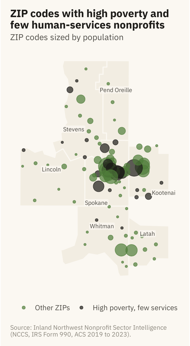
Figure 11.5
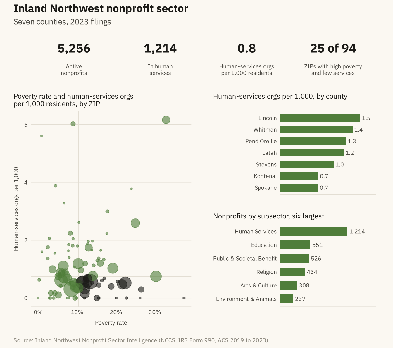
A one-page dashboard for the Inland Northwest nonprofit sector. Four numbers run across the top, the main chart is at the left, and two supporting charts are at the right. Every panel answers one question and uses the chapter’s one accent color. The first two tiles and the subsector bars count all 5,256 registered organizations. The per-1,000 tile, the county bars, and the scatter use the 711 human-services organizations with a ZIP code in the data. Source: Inland Northwest Nonprofit Sector Intelligence.
Code
tile <- function(value, label) {
  ggplot() + annotate("text", x = 0, y = 0.55, label = value, size = 5.5, family = mv_font(), fontface = "bold", color = mv_ink$ink) +
    annotate("text", x = 0, y = -0.5, label = label, size = 2.6, family = mv_font(), color = mv_ink$ink2, lineheight = 0.95) +
    scale_x_continuous(limits = c(-1, 1)) + scale_y_continuous(limits = c(-1.1, 1.3)) +
    coord_cartesian(clip = "off") + theme_void() + theme(plot.background = element_rect(fill = mv_ink$canvas, color = NA))
}
hs_zip <- gaps |> group_by(county) |> summarise(n_hs = sum(n_human_services), population = sum(population)) |>
  mutate(rate = 1000 * n_hs / population)
hs <- sum(orgs$subsector == "Human Services"); tot <- nrow(orgs)
k1 <- tile(label_comma()(tot), "Active\nnonprofits")
k2 <- tile(label_comma()(hs), "In human\nservices")
k3 <- tile(sprintf("%.1f", 1000 * sum(hs_zip$n_hs) / sum(hs_zip$population)), "Human-services orgs\nper 1,000 residents")
k4 <- tile(paste0(n_gap, " of ", nrow(g2)), "ZIPs with high poverty\nand few services")
main <- ggplot(g2, aes(poverty_rate, hs_per_1k)) +
  geom_hline(yintercept = median(g2$hs_per_1k), color = mv_ink$grid, linewidth = 0.5) +
  geom_vline(xintercept = median(g2$poverty_rate), color = mv_ink$grid, linewidth = 0.5) +
  geom_point(aes(size = population, color = gap), alpha = 0.6) +
  scale_color_manual(values = c(`TRUE` = mv_ink$ink, `FALSE` = mv_accent()), guide = "none") +
  scale_size_area(max_size = 9, guide = "none") +
  scale_x_continuous(labels = label_percent(scale = 1)) +
  labs(title = "Poverty rate and human-services orgs\nper 1,000 residents, by ZIP", x = "Poverty rate", y = "Human-services orgs per 1,000") +
  theme_mv(base_size = 9) + plain_title
cty_bar <- hs_zip |> mutate(county = fct_reorder(str_remove(county, " County"), rate))
side1 <- ggplot(cty_bar, aes(rate, county)) +
  geom_col(fill = mv_accent(), width = 0.65) +
  geom_text(aes(label = sprintf("%.1f", rate)), hjust = -0.2, size = 2.6, family = mv_font(), color = mv_ink$ink2) +
  scale_x_continuous(expand = expansion(mult = c(0, 0.2))) +
  labs(title = "Human-services orgs per 1,000, by county", x = NULL, y = NULL) +
  theme_mv(base_size = 9, grid = "none") + plain_title + theme(axis.text.x = element_blank())
sub <- orgs |> filter(subsector != "Unclassified") |> count(subsector, sort = TRUE) |> slice_head(n = 6) |>
  mutate(subsector = fct_reorder(subsector, n))
side2 <- ggplot(sub, aes(n, subsector)) +
  geom_col(fill = mv_accent(), width = 0.65) +
  geom_text(aes(label = label_comma()(n)), hjust = -0.2, size = 2.6, family = mv_font(), color = mv_ink$ink2) +
  scale_x_continuous(expand = expansion(mult = c(0, 0.45))) +
  labs(title = "Nonprofits by subsector, six largest", x = NULL, y = NULL) +
  theme_mv(base_size = 9, grid = "none") + plain_title + theme(axis.text.x = element_blank())
tiles <- (k1 | k2 | k3 | k4)
body <- (main | (side1 / side2)) + plot_layout(widths = c(5, 3))
(tiles / body) + plot_layout(heights = c(0.55, 2)) +
  plot_annotation(title = "Inland Northwest nonprofit sector", subtitle = "Seven counties, 2023 filings",
                  caption = mv_source(src),
                  theme = cap_theme + theme(plot.title = element_text(size = 14, face = "bold", family = mv_font(), color = mv_ink$ink),
                                            plot.subtitle = element_text(size = 10, family = mv_font(), color = mv_ink$ink2)))