# Where the data and the theme live. The defaults load from the companion
# site. Set MV_DATA and MV_THEME to local paths to work offline.
mv_data  <- Sys.getenv("MV_DATA",  "https://viz.marginoferrormedia.com/data")
mv_theme <- Sys.getenv("MV_THEME", "https://viz.marginoferrormedia.com/figures/mv-theme.R")Chapter 10: Uncertainty
The code behind every figure in Chapter 10 of Make It Visible, in the order the chapter draws them. Run the first chunk, then any figure. Each chunk stands on its own once the setup chunk has run.
Setup
Loads the theme, the packages, and the chapter’s data.
Code
source(mv_theme)
mv_set_chapter(10)
suppressPackageStartupMessages({ library(tidyverse); library(ggrepel); library(patchwork) })
polls <- read_csv(file.path(mv_data, "ch10-polls.csv"), show_col_types = FALSE)
pres <- polls |> filter(race_type == "Pres-G")
cap_theme <- theme(plot.caption = element_text(size = 7.5, hjust = 0, color = mv_ink$mute, family = mv_font()),
                   plot.background = element_rect(fill = mv_ink$canvas, color = NA))
plain_title <- theme(plot.title = element_text(size = rel(1), face = "plain"))
src <- "FiveThirtyEight pollster ratings database"
moe <- function(n, p = 0.5) 1.96 * sqrt(p * (1 - p) / n) * 100
# The single poll used in fig-ch10-onepoll. Every number quoted about it is computed here.
one <- pres |> filter(race == "2016_Pres-G_US", days_to_election <= 14, sample_size >= 1100, sample_size <= 1300) |>
  slice(1)
m_one <- one$margin_poll; n_one <- one$sample_size; e_one <- 2 * moe(n_one); a_one <- one$margin_actual
lo_one <- m_one - e_one; hi_one <- m_one + e_one
fmt1 <- function(x) sprintf("%.1f", x)
side <- function(x) if_else(x >= 0, paste0("Clinton +", fmt1(x)), paste0("Trump +", fmt1(-x)))
# Polls within 21 days, used by fig-ch10-errors, fig-ch10-sample and fig-ch10-lean
late <- pres |> filter(days_to_election <= 21, !is.na(error))
samp <- late |> filter(sample_size >= 200, sample_size <= 5000) |> mutate(above = abs(error) > 2 * moe(sample_size))
ab_lab <- c(mean(samp$above[samp$sample_size <= 500]), mean(samp$above[samp$sample_size > 3000])) |>
  (\(x) paste0(round(100 * x), " percent"))()
# Captions that quote computed numbers
cap_onepoll <- paste0("One national poll from October 2016, shown as a point (left), as a point with its 95 percent margin of error (center), and with the result added (right). The poll's range of plus or minus ", fmt1(moe(n_one)), " points on each candidate becomes a range of about ", fmt1(e_one), " points on the margin. That range covers the actual margin of ", fmt1(a_one), ", so the poll was within its stated error. Only the point form, without the range, makes the poll look wrong. Source: FiveThirtyEight pollster ratings database.")
cap_band <- paste0("National presidential polls in the last 60 days of the 2016 campaign (grey points), a smoothed average (line), and a band for the uncertainty in the average. The band is the uncertainty of the average, not the range where a single poll might fall. The result, Clinton by ", fmt1(a_one), ", is marked. Source: FiveThirtyEight pollster ratings database.")
cap_sample <- paste0("Absolute error in the margin against sample size for presidential polls within 21 days of the election, with samples of 200 to 5,000, and the sampling margin of error on the margin drawn as a curve. The curve falls steeply below 500 respondents and flattens after that. The typical error of the polls falls only a little as samples grow. The share of polls above the curve rises with sample size, from about ", ab_lab[1], " below 500 respondents to about ", ab_lab[2], " above 3,000. Source: FiveThirtyEight pollster ratings database.")
Figure 10.1
!expr cap_onepoll
Code
base <- function(title) ggplot() +
  scale_x_continuous(limits = c(-4, 12), breaks = c(-4, 0, 4, 8, 12), labels = \(x) if_else(x > 0, paste0("+", x), as.character(x))) +
  scale_y_continuous(limits = c(0.4, 1.6), breaks = NULL) +
  geom_vline(xintercept = 0, color = mv_ink$grid, linewidth = 0.5) +
  labs(x = NULL, y = NULL, title = title) + theme_mv(base_size = 10, grid = "none") + plain_title
p1 <- base(paste0("Point estimate:\n", side(m_one))) + annotate("point", x = m_one, y = 1, color = mv_accent(), size = 3.5)
p2 <- base(paste0("With a 95 percent interval:\n+", fmt1(m_one), ", plus or minus ", fmt1(e_one))) +
  annotate("segment", x = lo_one, xend = hi_one, y = 1, yend = 1, color = mv_accent(), linewidth = 1.2) +
  annotate("point", x = m_one, y = 1, color = mv_accent(), size = 3.5)
p3 <- base(paste0("With the result:\n", side(a_one))) +
  annotate("segment", x = lo_one, xend = hi_one, y = 1, yend = 1, color = mv_accent(), linewidth = 1.2) +
  annotate("point", x = m_one, y = 1, color = mv_accent(), size = 3.5) +
  annotate("point", x = a_one, y = 1, color = mv_ink$ink, shape = 18, size = 4) +
  annotate("text", x = a_one, y = 1.3, label = "Result", size = 2.8, family = mv_font(), color = mv_ink$ink)
p1 + p2 + p3 + plot_annotation(caption = mv_source(src, "Error on a margin is about twice the per-candidate error"), theme = cap_theme)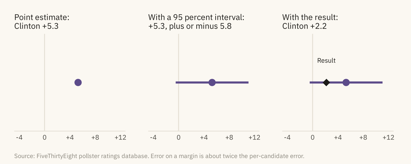
Figure 10.2
Error in the margin, poll minus result, for 2,900 presidential polls taken within 21 days of the election, 2000 to 2020. The shaded band is the sampling margin of error for a poll of 1,000, plus or minus 6 points on the margin. About a quarter of polls fall outside it. The center of the distribution is also above zero, so on average the polls overstated the Democratic candidate’s margin. Source: FiveThirtyEight pollster ratings database.
Code
share_out <- mean(abs(late$error) > 6)
ggplot(late, aes(error)) +
  annotate("rect", xmin = -6, xmax = 6, ymin = 0, ymax = Inf, fill = "#D9D3C5") +
  geom_histogram(binwidth = 1, boundary = 0, fill = mv_accent(), color = mv_ink$canvas, linewidth = 0.3) +
  geom_vline(xintercept = 0, color = mv_ink$ink, linewidth = 0.5) +
  annotate("text", x = 6.5, y = 300, label = paste0(percent(share_out, 1), " of polls fall outside\nthe sampling margin of error"),
           hjust = 0, vjust = 1, size = 2.9, family = mv_font(), color = mv_ink$ink2, lineheight = 0.95) +
  annotate("text", x = -6.5, y = 300, label = "Sampling error\nfor n = 1,000", hjust = 1, vjust = 1, size = 2.9, family = mv_font(), color = mv_ink$ink2, lineheight = 0.95) +
  scale_x_continuous(limits = c(-25, 25), breaks = seq(-20, 20, 10), labels = \(x) if_else(x > 0, paste0("+", x), as.character(x))) +
  scale_y_continuous(expand = expansion(mult = c(0, 0.05))) +
  labs(title = "Error in the margin for presidential polls, 2000 to 2020",
       subtitle = "Poll margin minus actual margin, presidential polls within 21 days of the election",
       x = "Poll margin minus actual margin, percentage points", y = "Polls", caption = mv_source(src)) +
  theme_mv()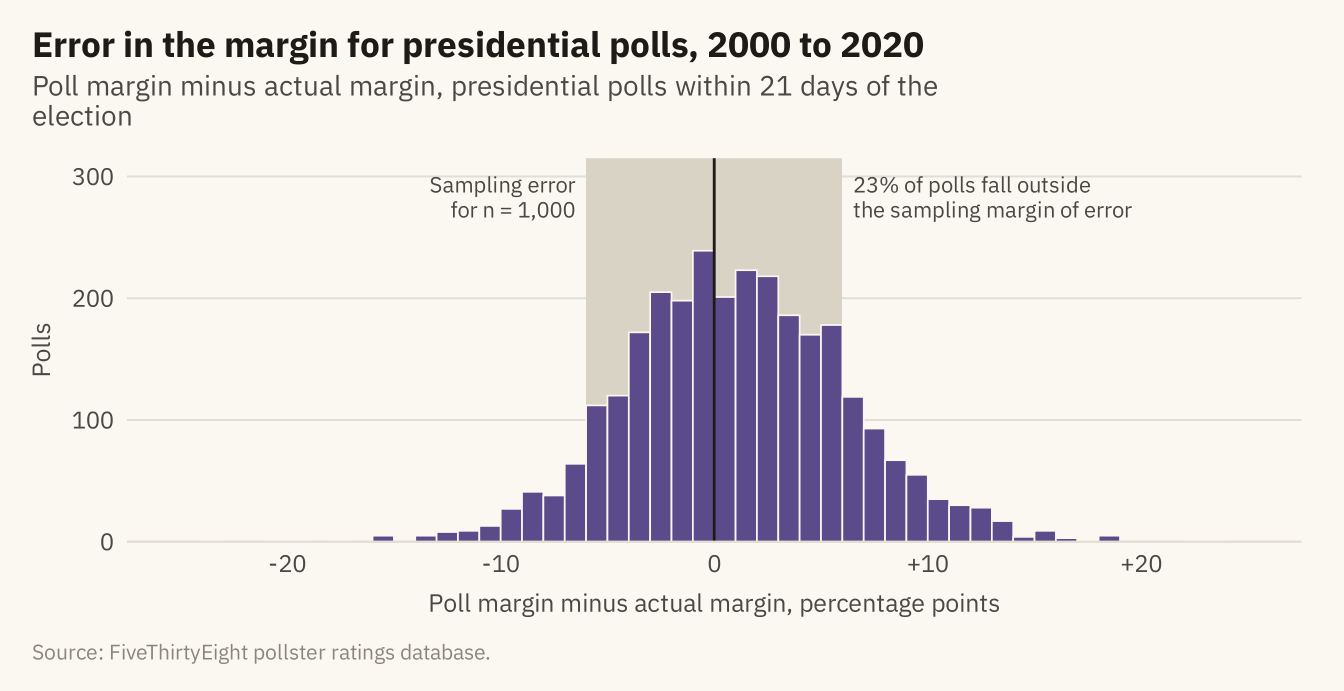
Figure 10.3
Four ways to show the same uncertainty. The average poll margin in twelve states in the last three weeks of 2020, with a 95 percent interval from the spread of polls, shown as a bar with error whiskers, a point with an interval, a gradient that fades with distance from the estimate, and a quantile dot plot in which each of twenty dots is an equally likely outcome. The dots are stacked in five rows so that they can be counted. The actual result is the black diamond. Source: FiveThirtyEight pollster ratings database.
Code
bg <- c("AZ", "GA", "WI", "PA", "NC", "MI", "NV", "FL", "TX", "OH", "MN", "IA")
s20 <- pres |> filter(cycle == 2020, state %in% bg, days_to_election <= 21) |>
  group_by(state) |> summarise(n = n(), est = mean(margin_poll), se = sd(margin_poll) / sqrt(n()),
                                actual = first(margin_actual), .groups = "drop") |>
  mutate(lo = est - 1.96 * se, hi = est + 1.96 * se, state = fct_reorder(state, est))
lab_x <- scale_x_continuous(limits = c(-14, 14), breaks = c(-10, 0, 10), labels = \(x) if_else(x > 0, paste0("D+", x), if_else(x < 0, paste0("R+", -x), "Even")))
# The result diamond, drawn with a thin canvas outline so it stays visible over bars and gradients
result_pt <- geom_point(data = s20, aes(actual, state), shape = 23, size = 2.4, fill = mv_ink$ink, color = mv_ink$canvas, stroke = 0.4)
f1 <- ggplot(s20, aes(est, state)) +
  geom_col(fill = mv_accent(), width = 0.6, alpha = 0.7) +
  geom_errorbar(aes(xmin = lo, xmax = hi), width = 0.3, color = mv_ink$ink, linewidth = 0.4) +
  result_pt +
  geom_vline(xintercept = 0, color = mv_ink$mute, linewidth = 0.4) + lab_x +
  labs(x = NULL, y = NULL, title = "Bars with whiskers") + theme_mv(base_size = 10, grid = "x") + plain_title
f2 <- ggplot(s20, aes(est, state)) +
  geom_segment(aes(x = lo, xend = hi, yend = state), color = mv_accent(), linewidth = 1.2) +
  geom_point(color = mv_accent(), size = 2.4) +
  result_pt +
  geom_vline(xintercept = 0, color = mv_ink$mute, linewidth = 0.4) + lab_x +
  labs(x = NULL, y = NULL, title = "Point and interval") + theme_mv(base_size = 10, grid = "x") + plain_title
grad <- s20 |> crossing(k = seq(-2.5, 2.5, length.out = 201)) |>
  mutate(x = est + k * se, w = dnorm(k) / dnorm(0),
         fill = colorRampPalette(c(mv_ink$canvas, mv_accent()))(101)[round(w * 100) + 1])
f3 <- ggplot(grad, aes(x, state)) +
  geom_tile(aes(fill = fill, color = fill, width = 5 * se / 200), height = 0.75, linewidth = 0.25) +
  scale_fill_identity() + scale_color_identity() +
  result_pt +
  geom_vline(xintercept = 0, color = mv_ink$mute, linewidth = 0.4) + lab_x +
  labs(x = NULL, y = NULL, title = "Gradient") + theme_mv(base_size = 10, grid = "x") + plain_title
# Twenty quantiles per state, stacked in five rows in order of value so neighbouring dots do not overlap
qd <- s20 |> crossing(i = 1:20) |> mutate(q = (i - 0.5) / 20, x = qnorm(q, est, se), row = ((i - 1) %% 5 - 2) * 0.17)
f4 <- ggplot(qd, aes(x, as.numeric(state) + row)) +
  geom_point(color = mv_accent(), size = 0.55) +
  scale_y_continuous(breaks = seq_along(levels(s20$state)), labels = levels(s20$state), limits = c(0.4, 12.6)) +
  geom_point(data = s20, aes(actual, as.numeric(state)), shape = 23, size = 2.4, fill = mv_ink$ink, color = mv_ink$canvas, stroke = 0.4) +
  geom_vline(xintercept = 0, color = mv_ink$mute, linewidth = 0.4) + lab_x +
  labs(x = NULL, y = NULL, title = "Twenty possible outcomes") + theme_mv(base_size = 10, grid = "x") + plain_title
f1 / f2 / f3 / f4 + plot_annotation(caption = mv_source(src, "Interval from the spread of polls in each state"), theme = cap_theme)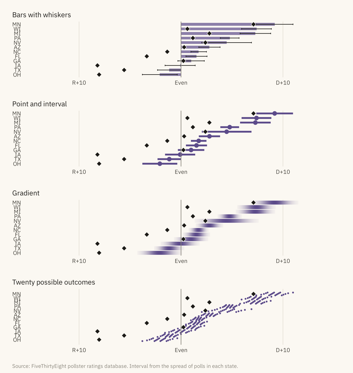
Figure 10.4
!expr cap_band
Code
n16 <- pres |> filter(race == "2016_Pres-G_US", days_to_election <= 70)
ggplot(n16, aes(-days_to_election, margin_poll)) +
  geom_hline(yintercept = 0, color = mv_ink$mute, linewidth = 0.4) +
  geom_point(color = mv_ink$mute, size = 1, alpha = 0.4) +
  geom_smooth(method = "loess", span = 0.3, color = mv_accent(), fill = mv_accent(), alpha = 0.2, linewidth = 1, formula = y ~ x) +
  annotate("point", x = 0, y = a_one, shape = 18, size = 4, color = mv_ink$ink) +
  annotate("text", x = 1.5, y = a_one, label = paste0("Result:\n+", fmt1(a_one)), hjust = 0, vjust = 0.5, size = 2.9, family = mv_font(), color = mv_ink$ink, lineheight = 0.9) +
  scale_x_continuous(breaks = c(-60, -30, 0), labels = c("60 days out", "30 days out", "Election"), limits = c(-61, 9)) +
  scale_y_continuous(breaks = seq(-5, 15, 5), labels = \(x) if_else(x > 0, paste0("Clinton +", x), if_else(x < 0, paste0("Trump +", -x), "Even"))) +
  labs(title = "National polls and smoothed average, last 60 days of the 2016 campaign",
       subtitle = "Clinton minus Trump, percentage points, with a band for the uncertainty of the average",
       x = NULL, y = NULL, caption = mv_source(src)) +
  theme_mv()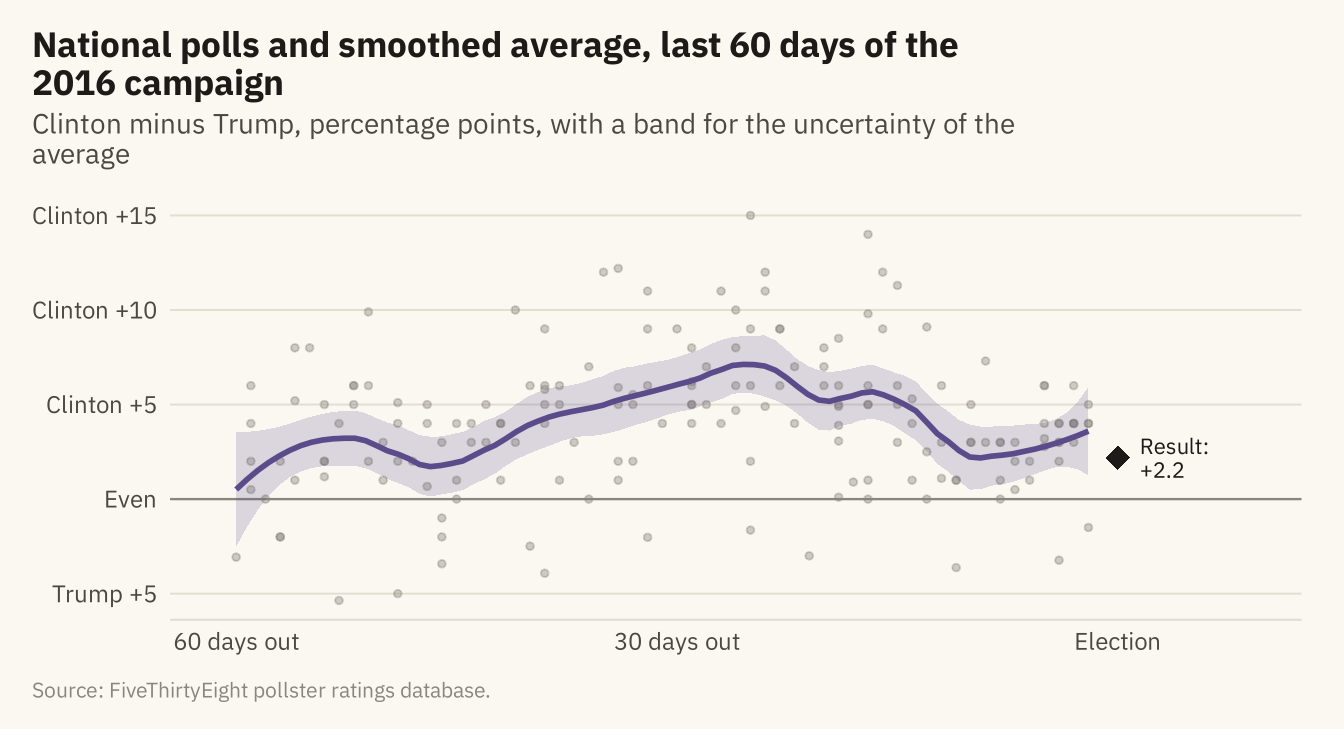
Figure 10.5
!expr cap_sample
Code
curve <- tibble(n = seq(200, 5000, 50), e = 2 * moe(n))
ggplot(samp, aes(sample_size, abs(error))) +
  geom_point(color = mv_accent(), size = 0.9, alpha = 0.3) +
  geom_line(data = curve, aes(n, e), color = mv_ink$ink, linewidth = 0.9) +
  annotate("label", x = 3600, y = 8.5, label = "Sampling margin of error\n(95 percent, on the margin)", hjust = 0, size = 2.8,
           family = mv_font(), color = mv_ink$ink, fill = mv_ink$canvas, label.size = 0, lineheight = 0.95) +
  scale_x_continuous(labels = label_comma()) +
  scale_y_continuous(limits = c(0, 25), expand = expansion(0)) +
  labs(title = "Absolute error in the margin by sample size, presidential polls, 2000 to 2020",
       subtitle = "Each point is one poll within 21 days of the election. Curve: sampling margin of error",
       x = "Sample size", y = "Absolute error, points", caption = mv_source(src)) +
  theme_mv(grid = "y") + theme(panel.grid.major.x = element_line(color = mv_ink$grid, linewidth = 0.35))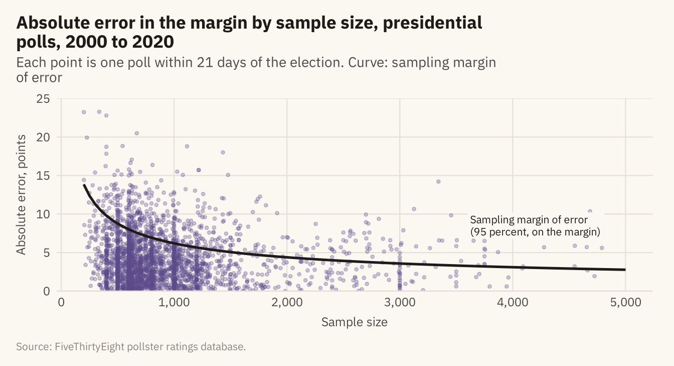
Figure 10.6
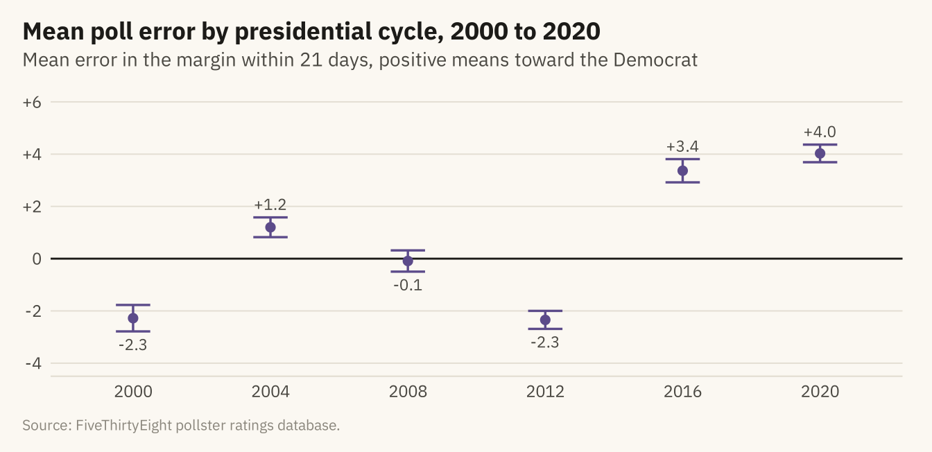
Mean error in the margin, poll minus result, across presidential polls in the final 21 days of each cycle from 2000 to 2020, with 95 percent intervals. A positive value means polls leaned toward the Democrat. The lean changes sign across cycles and was largest in 2016 and 2020. Source: FiveThirtyEight pollster ratings database.
Code
lean <- late |> group_by(cycle) |> summarise(n = n(), m = mean(error), se = sd(error) / sqrt(n()), .groups = "drop") |>
  mutate(lo = m - 1.96 * se, hi = m + 1.96 * se)
ggplot(lean, aes(factor(cycle), m)) +
  geom_hline(yintercept = 0, color = mv_ink$ink, linewidth = 0.5) +
  geom_errorbar(aes(ymin = lo, ymax = hi), color = mv_accent(), width = 0.25, linewidth = 0.6) +
  geom_point(color = mv_accent(), size = 2) +
  geom_text(aes(label = sprintf("%+.1f", m), y = if_else(m > 0, hi + 0.5, lo - 0.5)), size = 3, family = mv_font(), color = mv_ink$ink2) +
  scale_y_continuous(limits = c(-4, 6), breaks = seq(-4, 6, 2), labels = \(x) if_else(x > 0, paste0("+", x), as.character(x))) +
  labs(title = "Mean poll error by presidential cycle, 2000 to 2020",
       subtitle = "Mean error in the margin within 21 days, positive means toward the Democrat",
       x = NULL, y = NULL, caption = mv_source(src)) +
  theme_mv()