# Where the data and the theme live. The defaults load from the companion
# site. Set MV_DATA and MV_THEME to local paths to work offline.
mv_data  <- Sys.getenv("MV_DATA",  "https://viz.marginoferrormedia.com/data")
mv_theme <- Sys.getenv("MV_THEME", "https://viz.marginoferrormedia.com/figures/mv-theme.R")Chapter 9: Color, Type, and Annotation
The code behind every figure in Chapter 9 of Make It Visible, in the order the chapter draws them. Run the first chunk, then any figure. Each chunk stands on its own once the setup chunk has run.
Setup
Loads the theme, the packages, and the chapter’s data.
Code
source(mv_theme)
mv_set_chapter(9)
suppressPackageStartupMessages({ library(tidyverse); library(ggrepel); library(patchwork) })
us <- read_csv(file.path(mv_data, "ch09-trust-us.csv"), show_col_types = FALSE)
wv <- read_csv(file.path(mv_data, "ch09-trust-world.csv"), show_col_types = FALSE)
cap_theme <- theme(plot.caption = element_text(size = 7.5, hjust = 0, color = mv_ink$mute, family = mv_font()),
                   plot.background = element_rect(fill = mv_ink$canvas, color = NA))
plain_title <- theme(plot.title = element_text(size = rel(1), face = "plain"))
src_us <- "General Social Survey, via Our World in Data"
src_wv <- "World Values Survey, via Our World in Data"
ten <- c("Sweden", "Netherlands", "Germany", "Japan", "United States", "South Korea", "Mexico", "Brazil", "Colombia", "Philippines")
wv10 <- wv |> filter(country %in% ten, year >= 1990)
# Simulate deuteranopia with the Machado, Oliveira, and Fernandes (2009) matrix at full severity.
deutan <- function(hex) {
  M <- matrix(c(0.367322, 0.860646, -0.227968, 0.280085, 0.672501, 0.047413, -0.011820, 0.042940, 0.968881), 3, byrow = TRUE)
  rgb <- grDevices::col2rgb(hex) / 255
  out <- pmin(pmax(M %*% rgb, 0), 1)
  setNames(grDevices::rgb(out[1, ], out[2, ], out[3, ]), names(hex))
}
Figure 9.1
Share of people saying most people can be trusted, ten countries, World Values Survey waves since 1990, drawn with library defaults. The chart has ten hues, a legend, a grey panel, and a title that names the topic rather than a finding. Source: World Values Survey, via Our World in Data.
Code
old <- options(ggplot2.discrete.colour = NULL, ggplot2.discrete.fill = NULL)
ggplot(wv10, aes(year, trust, color = country)) +
  geom_line() + geom_point() +
  labs(x = "year", y = "trust", color = "country", title = "Trust by country")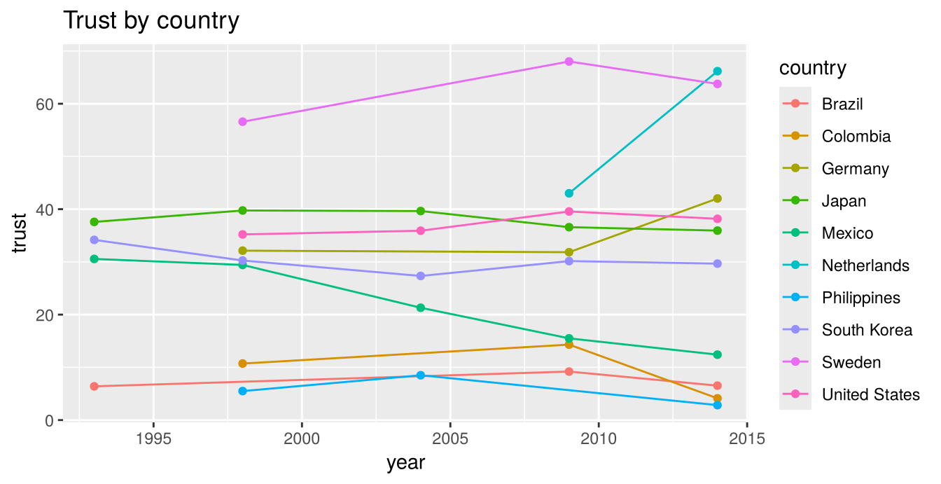
Code
options(old)Figure 9.2
The same data after the color, type, and annotation have been chosen. One accent marks the United States, the other countries are grey, each line has a direct label, the title states the finding, and one annotation describes the series at the top. Source: World Values Survey, via Our World in Data.
Code
ends <- wv10 |> group_by(country) |> slice_max(year, n = 1) |> ungroup()
ggplot(wv10, aes(year, trust, group = country)) +
  geom_line(data = filter(wv10, country != "United States"), color = "#C9C3B6", linewidth = 0.8) +
  geom_line(data = filter(wv10, country == "United States"), color = mv_accent(), linewidth = 1.2) +
  geom_point(data = filter(wv10, country == "United States"), color = mv_accent(), size = 2) +
  mv_label_end(filter(ends, country != "United States"), aes(label = country), color = mv_ink$mute, nudge_x = 0.4, size = 2.8) +
  mv_label_end(filter(ends, country == "United States"), aes(label = country), color = mv_accent(), nudge_x = 0.4, size = 3) +
  annotate("text", x = 1991, y = 72, label = "Sweden is above 55 percent in every wave it appears in", hjust = 0,
           size = 2.9, family = mv_font(), color = mv_ink$ink2) +
  scale_x_continuous(breaks = c(1990, 2000, 2010, 2014), limits = c(1990, 2021), expand = expansion(mult = 0.01)) +
  scale_y_continuous(labels = label_percent(scale = 1), limits = c(0, 80), expand = expansion(0)) +
  labs(title = "Americans trust each other less than most rich countries do",
       subtitle = "Share saying most people can be trusted, World Values Survey waves since 1990",
       x = NULL, y = NULL, caption = mv_source(src_wv)) +
  theme_mv()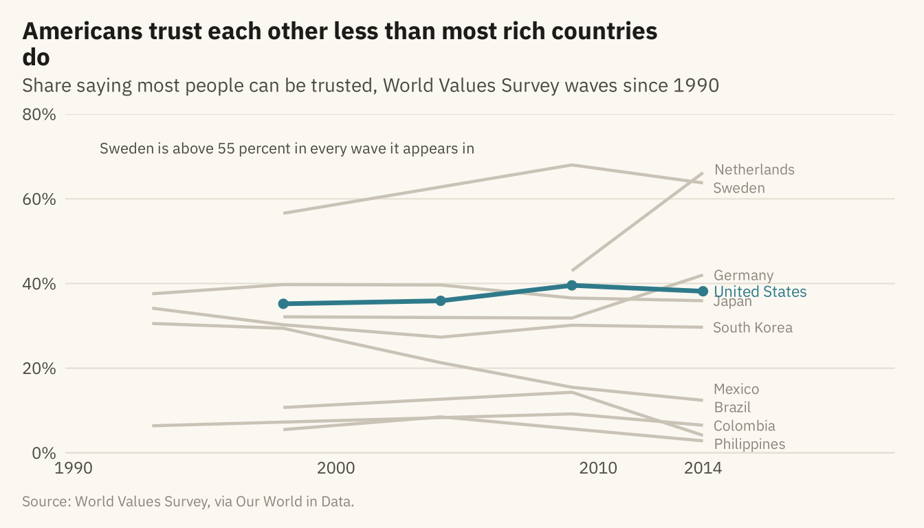
Figure 9.3
Three ways to color ten series. Left, ten hues, which a reader cannot match to countries without a legend. Center, four hues for the countries the chart is about and grey for the rest. Right, one accent and grey, for a chart that makes one point. Source: World Values Survey, via Our World in Data.
Code
h1 <- ggplot(wv10, aes(year, trust, color = country)) + geom_line(linewidth = 0.8) +
  scale_color_manual(values = colorRampPalette(c(mv_accent(), "#1C1B18", "#C9A227", "#5B6E8C", "#2E6B5E", "#A23B2C", "#7A4E8C", "#C25B2A", "#3C5A99", "#8C3A5E"))(10), guide = "none") +
  scale_x_continuous(limits = c(1990, 2022)) +
  scale_y_continuous(limits = c(0, 80)) + labs(x = NULL, y = NULL, title = "Ten hues") + theme_mv(base_size = 10) + plain_title
four <- c("Sweden", "United States", "Japan", "Brazil")
h2 <- ggplot(wv10, aes(year, trust, group = country)) +
  geom_line(data = filter(wv10, !country %in% four), color = "#C9C3B6", linewidth = 0.8) +
  geom_line(data = filter(wv10, country %in% four), aes(color = country), linewidth = 1) +
  mv_label_end(filter(ends, country %in% four), aes(label = country, color = country), nudge_x = 0.3, size = 2.6) +
  scale_color_manual(values = c(Sweden = "#2E6B5E", `United States` = mv_accent(), Japan = "#1C1B18", Brazil = "#C25B2A"), guide = "none") +
  scale_x_continuous(limits = c(1990, 2022)) + scale_y_continuous(limits = c(0, 80)) +
  labs(x = NULL, y = NULL, title = "Four hues and grey") + theme_mv(base_size = 10) + plain_title
h3 <- ggplot(wv10, aes(year, trust, group = country)) +
  geom_line(data = filter(wv10, country != "United States"), color = "#C9C3B6", linewidth = 0.8) +
  geom_line(data = filter(wv10, country == "United States"), color = mv_accent(), linewidth = 1.2) +
  mv_label_end(filter(ends, country == "United States"), aes(label = country), color = mv_accent(), nudge_x = 0.3, size = 2.6) +
  scale_x_continuous(limits = c(1990, 2022)) + scale_y_continuous(limits = c(0, 80)) +
  labs(x = NULL, y = NULL, title = "One accent and grey") + theme_mv(base_size = 10) + plain_title
h1 + h2 + h3 + plot_annotation(caption = mv_source(src_wv), theme = cap_theme)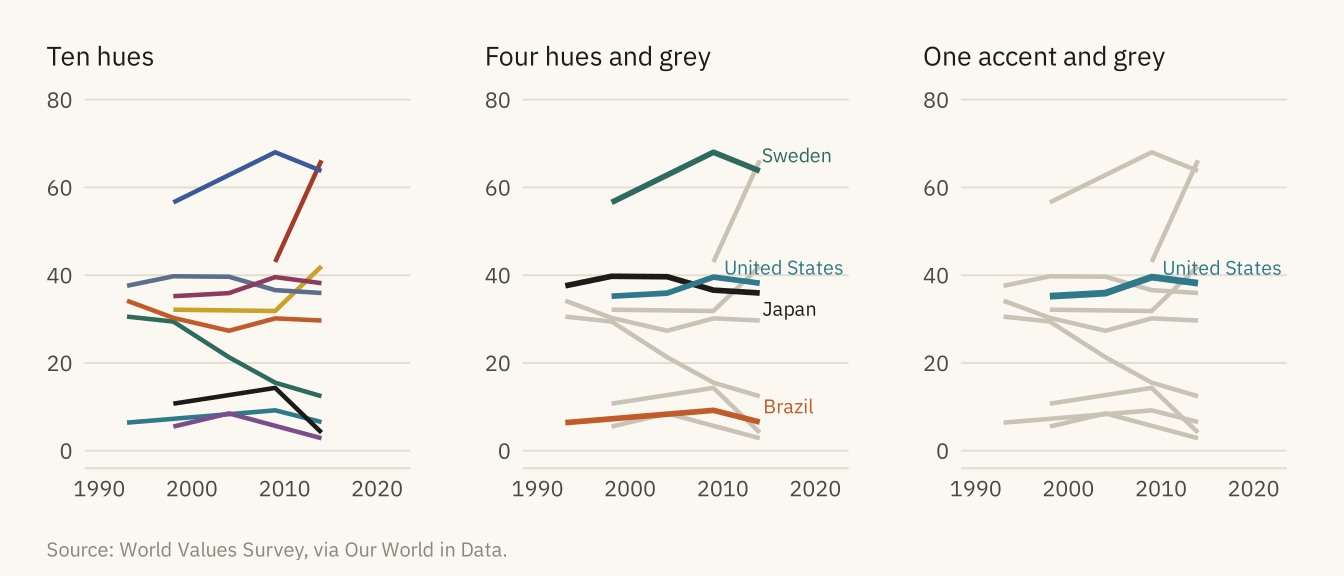
Figure 9.4
Two palettes for four countries, as seen with typical color vision (top) and as simulated for deuteranopia, the most common red-green deficiency (bottom). In the simulation, the red and green on the left become two shades of the same olive. The colors on the right differ in lightness as well as hue, so a reader can still tell them apart. Source: World Values Survey, via Our World in Data; simulation after Machado, Oliveira, and Fernandes (2009).
Code
wv4 <- filter(wv10, country %in% four)
e4 <- filter(ends, country %in% four)
pal_bad <- c(Sweden = "#2CA02C", `United States` = "#D62728", Japan = "#1F77B4", Brazil = "#FF7F0E")
pal_good <- c(Sweden = "#1C1B18", `United States` = mv_accent(), Japan = mv_ink$mute, Brazil = "#C9A227")
cvd <- function(pal, title) {
  ggplot(wv4, aes(year, trust, color = country)) + geom_line(linewidth = 1.1) +
    mv_label_end(e4, aes(label = country, color = country), nudge_x = 0.3, size = 2.5) +
    scale_color_manual(values = pal, guide = "none") +
    scale_x_continuous(limits = c(1990, 2024)) + scale_y_continuous(limits = c(0, 80)) +
    labs(x = NULL, y = NULL, title = title) + theme_mv(base_size = 9) + plain_title +
    theme(axis.text = element_blank())
}
(cvd(pal_bad, "Red and green, typical vision") + cvd(pal_good, "Lightness steps, typical vision")) /
  (cvd(deutan(pal_bad), "Red and green, deuteranopia") + cvd(deutan(pal_good), "Lightness steps, deuteranopia")) +
  plot_annotation(caption = mv_source(src_wv), theme = cap_theme)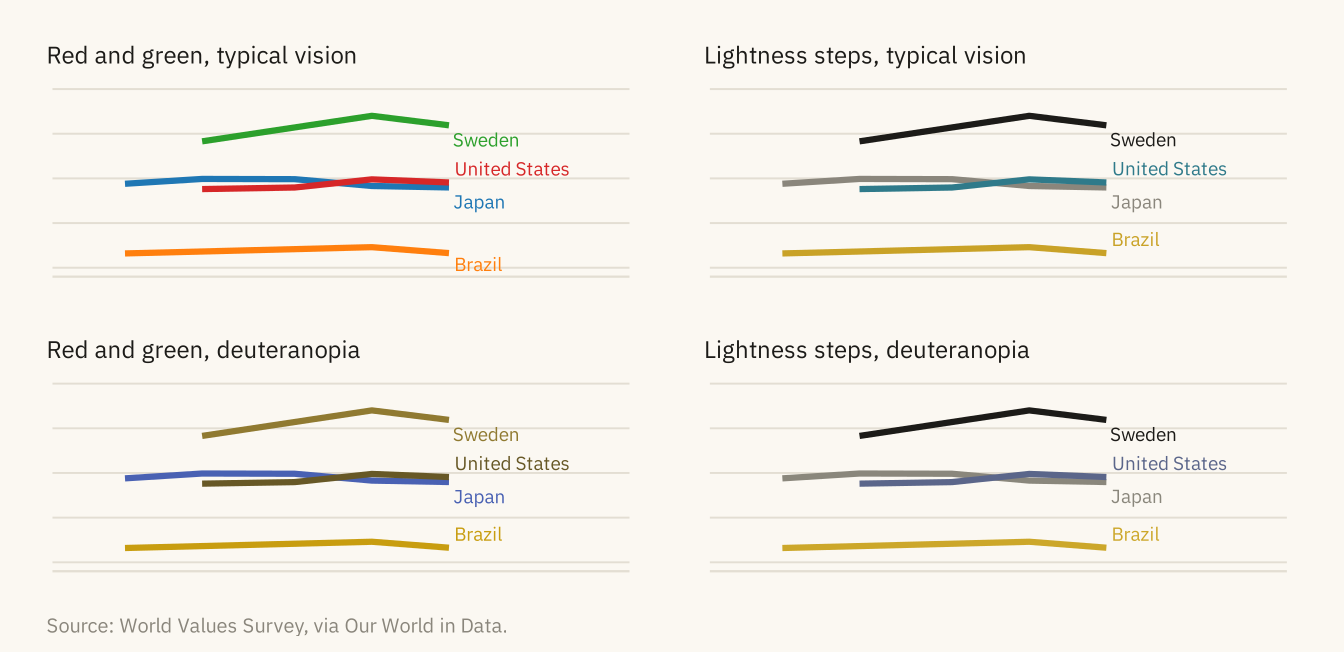
Figure 9.5
The American trust series with three treatments of type. Left, every element is the same size and weight, so nothing is read first. Center, too many sizes, weights, and faces, so the red title and the bold axis title are read before the subtitle that says what is measured. Right, three levels. The bold title states the finding, the lighter subtitle says what is measured, and small grey text covers the axes and source. Source: General Social Survey, via Our World in Data.
Code
base <- ggplot(us, aes(year, trust)) + geom_line(color = mv_accent(), linewidth = 1) +
  scale_y_continuous(labels = label_percent(scale = 1), limits = c(0, 60), expand = expansion(0)) +
  scale_x_continuous(breaks = c(1972, 1990, 2010))
t1 <- base + labs(title = "Trust fell by a third", subtitle = "Share saying most people\ncan be trusted", x = "Year", y = "Percent") +
  theme_minimal(base_size = 10, base_family = mv_font()) +
  theme(plot.title = element_text(size = 10, face = "plain"), plot.subtitle = element_text(size = 10), plot.title.position = "plot",
        axis.title = element_text(size = 10), axis.text = element_text(size = 10),
        plot.background = element_rect(fill = mv_ink$canvas, color = NA), panel.grid.minor = element_blank())
t2 <- base + labs(title = "TRUST FELL", subtitle = "Share saying most people\ncan be trusted", x = "YEAR", y = "Percent") +
  theme_minimal(base_size = 10, base_family = "serif") +
  theme(plot.title = element_text(size = 12, face = "bold.italic", family = "sans", color = "#B00020"),
        plot.subtitle = element_text(size = 9.5, face = "italic"), plot.title.position = "plot",
        axis.title.x = element_text(size = 12, face = "bold", family = "mono"), axis.title.y = element_text(size = 8),
        axis.text = element_text(size = 11, face = "bold"), plot.background = element_rect(fill = mv_ink$canvas, color = NA),
        panel.grid.minor = element_blank())
t3 <- base + labs(title = "Trust fell by a third", subtitle = "Share saying most people\ncan be trusted", x = NULL, y = NULL) +
  theme_mv(base_size = 10)
t1 + t2 + t3 + plot_annotation(caption = mv_source(src_us), theme = cap_theme)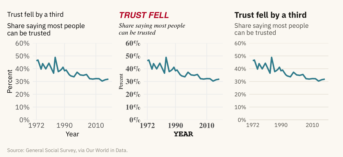
Figure 9.6
The American trust series with no annotation, with the start and end values marked, with the change named, and with the change named and the long flat stretch explained. Each addition gives the reader more guidance about what to look at. None changes the data. Source: General Social Survey, via Our World in Data.
Code
pts <- us |> filter(year %in% c(1972, 2018))
a0 <- base + labs(x = NULL, y = NULL, title = "Data only") + theme_mv(base_size = 10) + plain_title
a1 <- base + geom_point(data = pts, color = mv_accent(), size = 2.2) +
  geom_text(data = pts, aes(label = paste0(round(trust), "%"), hjust = c(0, 1)), vjust = -1, size = 3, family = mv_font(), color = mv_ink$ink2) +
  labs(x = NULL, y = NULL, title = "Values at the ends") + theme_mv(base_size = 10) + plain_title
a2 <- a1 + annotate("segment", x = 2021, xend = 2021, y = 31.8, yend = 46.2, color = mv_ink$ink, linewidth = 0.5,
                    arrow = arrow(ends = "both", length = unit(0.12, "cm"))) +
  annotate("text", x = 2023, y = 39, label = "Down 14\npoints", hjust = 0, size = 2.8, family = mv_font(), color = mv_ink$ink, lineheight = 0.9) +
  scale_x_continuous(breaks = c(1972, 1990, 2010), limits = c(1972, 2036)) +
  labs(title = "The change named") + plain_title
a3 <- a2 + labs(title = "The pattern explained") + plain_title
a3$layers <- c(list(annotate("rect", xmin = 1994, xmax = 2018, ymin = 0, ymax = 60, fill = mv_ink$grid, alpha = 0.4)), a3$layers)
a3 <- a3 + annotate("text", x = 2006, y = 54, label = "Flat for a generation:\nthe fall came before 1994", size = 2.8,
                    family = mv_font(), color = mv_ink$ink2, lineheight = 0.9)
(a0 + a1) / (a2 + a3) + plot_annotation(caption = mv_source(src_us), theme = cap_theme)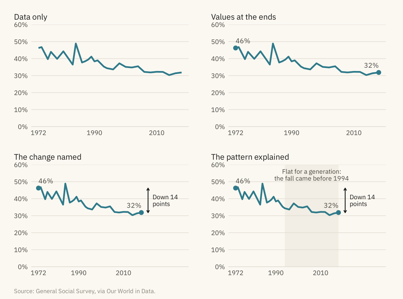
Figure 9.7
Four countries with a legend (left) and with direct labels at the end of each line (right). With the legend, the reader has to match four colors between the box and the lines. With direct labels, no matching is needed. Source: World Values Survey, via Our World in Data.
Code
l1 <- ggplot(wv4, aes(year, trust, color = country)) + geom_line(linewidth = 1) +
  scale_color_manual(values = pal_good, name = NULL) +
  scale_y_continuous(limits = c(0, 80)) +
  labs(x = NULL, y = NULL, title = "Legend") + theme_mv(base_size = 10) + plain_title +
  theme(legend.position = "right")
l2 <- ggplot(wv4, aes(year, trust, color = country)) + geom_line(linewidth = 1) +
  mv_label_end(e4, aes(label = country, color = country), nudge_x = 0.3, size = 2.8) +
  scale_color_manual(values = pal_good, guide = "none") +
  scale_x_continuous(limits = c(1990, 2024)) + scale_y_continuous(limits = c(0, 80)) +
  labs(x = NULL, y = NULL, title = "Direct labels") + theme_mv(base_size = 10) + plain_title
l1 + l2 + plot_annotation(caption = mv_source(src_wv), theme = cap_theme)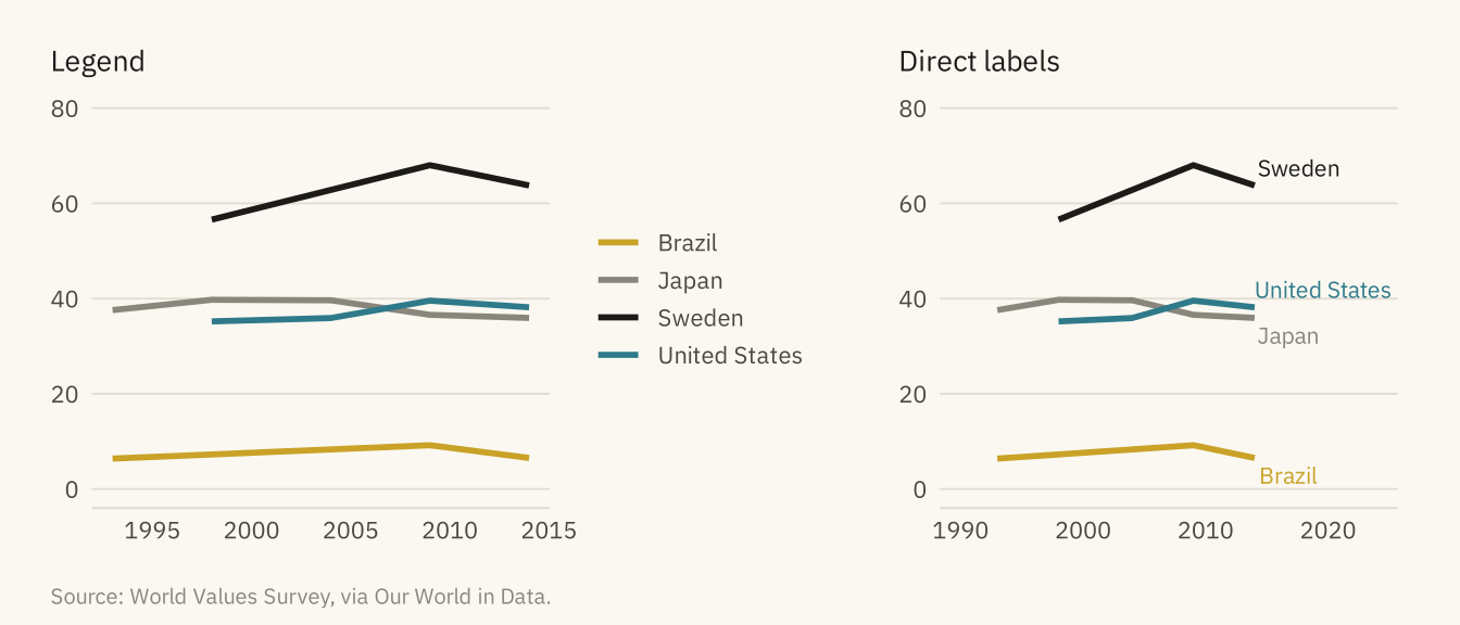
Figure 9.8
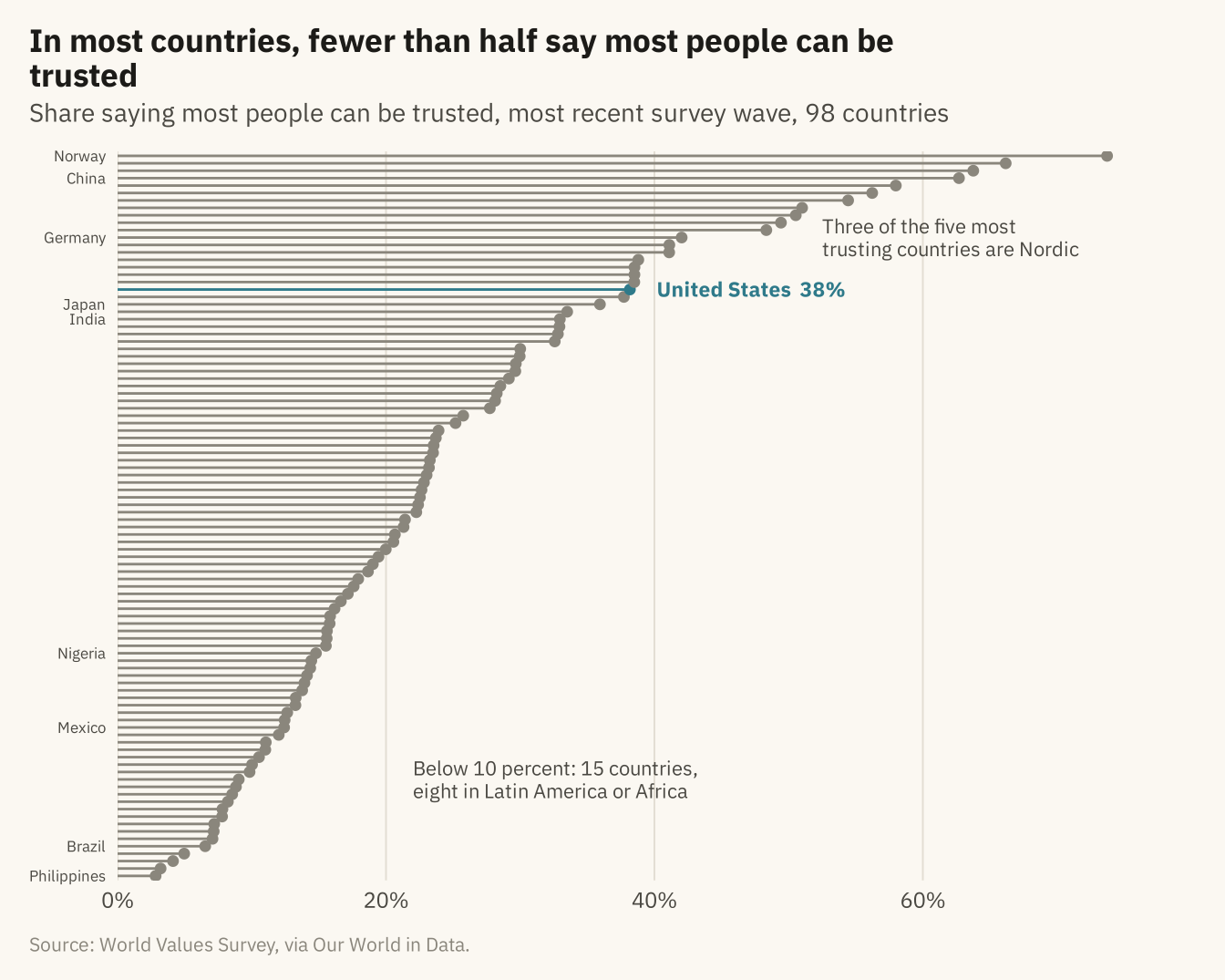
Share saying most people can be trusted in the most recent World Values Survey wave for each country, 98 countries sorted by value. The United States is marked. The Nordic countries, the Netherlands, and China are near the top. Most of Latin America and much of Africa are near the bottom. Source: World Values Survey, via Our World in Data.
Code
latest <- wv |> group_by(country) |> slice_max(year, n = 1) |> ungroup() |>
  mutate(country = fct_reorder(country, trust), us_flag = country == "United States")
ggplot(latest, aes(trust, country)) +
  geom_segment(aes(x = 0, xend = trust, yend = country, color = us_flag), linewidth = 0.5) +
  geom_point(aes(color = us_flag), size = 1.6) +
  geom_text(data = filter(latest, us_flag), aes(label = paste0("United States  ", round(trust), "%")),
            hjust = 0, nudge_x = 2, size = 3, family = mv_font(), color = mv_accent(), fontface = "bold") +
  annotate("text", x = 52.5, y = 87, label = "Three of the five most\ntrusting countries are Nordic", hjust = 0,
           size = 2.9, family = mv_font(), color = mv_ink$ink2, lineheight = 0.95) +
  annotate("text", x = 22, y = 14, label = "Below 10 percent: 15 countries,\neight in Latin America or Africa", hjust = 0,
           size = 2.9, family = mv_font(), color = mv_ink$ink2, lineheight = 0.95) +
  scale_color_manual(values = c(`TRUE` = mv_accent(), `FALSE` = mv_ink$mute), guide = "none") +
  scale_x_continuous(labels = label_percent(scale = 1), expand = expansion(mult = c(0, 0.08))) +
  scale_y_discrete(labels = \(x) if_else(x %in% c("Norway", "China", "Germany", "Japan", "India",
                                                   "Mexico", "Nigeria", "Brazil", "Philippines"), x, "")) +
  labs(title = "In most countries, fewer than half say most people can be trusted",
       subtitle = "Share saying most people can be trusted, most recent survey wave, 98 countries",
       x = NULL, y = NULL, caption = mv_source(src_wv)) +
  theme_mv(grid = "x") +
  theme(axis.text.y = element_text(size = rel(0.7)), panel.grid.major.y = element_blank())