# Where the data and the theme live. The defaults load from the companion
# site. Set MV_DATA and MV_THEME to local paths to work offline.
mv_data  <- Sys.getenv("MV_DATA",  "https://viz.marginoferrormedia.com/data")
mv_theme <- Sys.getenv("MV_THEME", "https://viz.marginoferrormedia.com/figures/mv-theme.R")Chapter 7: Change Over Time
The code behind every figure in Chapter 7 of Make It Visible, in the order the chapter draws them. Run the first chunk, then any figure. Each chunk stands on its own once the setup chunk has run.
Setup
Loads the theme, the packages, and the chapter’s data.
Code
source(mv_theme)
mv_set_chapter(7)
suppressPackageStartupMessages({ library(tidyverse); library(ggrepel); library(patchwork) })
nat <- read_csv(file.path(mv_data, "ch07-incarceration-national.csv"), show_col_types = FALSE) |> filter(year <= 2015)
st  <- read_csv(file.path(mv_data, "ch07-incarceration-state.csv"), show_col_types = FALSE) |> filter(year <= 2015)
cap_theme <- theme(plot.caption = element_text(size = 7.5, hjust = 0, color = mv_ink$mute, family = mv_font()),
                   plot.background = element_rect(fill = mv_ink$canvas, color = NA))
plain_title <- theme(plot.title = element_text(size = rel(1), face = "plain"))
src <- "Vera Institute of Justice, Incarceration Trends"
jail <- nat |> filter(jail_reported > 3000)
prison <- nat |> filter(year >= 1983, year <= 2013)
Figure 7.1
People held in county jails on a single day each year, 1970 to 2015, summed across about 3,070 counties. The count was flat through the 1970s, tripled between 1980 and 2000, and peaked in 2008. It has stayed below the peak since, with a small rise in 2012 and 2013. Source: Vera Institute of Justice, Incarceration Trends.
Code
peak <- jail |> slice_max(jail, n = 1)
ggplot(jail, aes(year, jail)) +
  geom_area(fill = mv_accent(), alpha = 0.12) +
  geom_line(color = mv_accent(), linewidth = 1.1) +
  geom_point(data = peak, color = mv_accent(), size = 2.4) +
  annotate("text", x = peak$year, y = peak$jail, label = paste0("Peak, ", peak$year, ": ", label_comma()(round(peak$jail, -3))),
           vjust = -1, hjust = 1, size = 3, family = mv_font(), color = mv_ink$ink2) +
  scale_x_continuous(breaks = seq(1970, 2015, 5), expand = expansion(mult = 0.01)) +
  scale_y_continuous(labels = label_comma(), limits = c(0, 900000), expand = expansion(0)) +
  labs(title = "Jail population, 1970 to 2015",
       subtitle = "People held in county jails on a single day, summed across counties",
       x = NULL, y = NULL, caption = mv_source(src)) +
  theme_mv()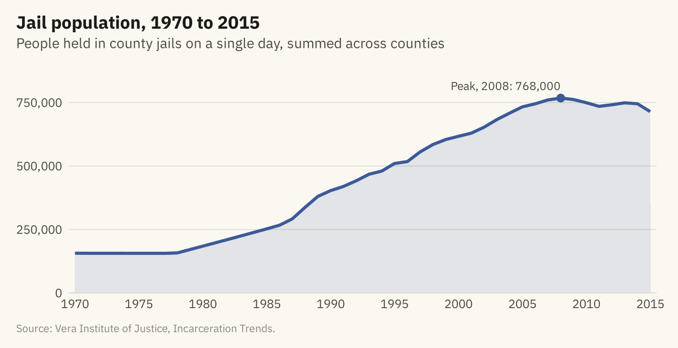
Figure 7.2
The jail count (left) and the jail rate per 100,000 residents aged 15 to 64 (right), 1970 to 2015. The rate rose almost as fast as the count, so most of the rise in the count is not explained by growth in the population. A chart of counts should be checked against the rate before a reader draws a conclusion. Source: Vera Institute of Justice, Incarceration Trends.
Code
cnt <- ggplot(jail, aes(year, jail)) +
  geom_line(color = mv_accent(), linewidth = 1) +
  scale_x_continuous(breaks = c(1970, 1990, 2010)) +
  scale_y_continuous(labels = label_comma(scale = 1e-3, suffix = "k"), limits = c(0, NA), expand = expansion(mult = c(0, 0.05))) +
  labs(x = NULL, y = NULL, title = "Count: people in jail") + theme_mv(base_size = 10) + plain_title
rt <- ggplot(jail, aes(year, jail_rate)) +
  geom_line(color = mv_accent(), linewidth = 1) +
  scale_x_continuous(breaks = c(1970, 1990, 2010)) +
  scale_y_continuous(limits = c(0, NA), expand = expansion(mult = c(0, 0.05))) +
  labs(x = NULL, y = NULL, title = "Rate: per 100,000 adults") + theme_mv(base_size = 10) + plain_title
cnt + rt + plot_annotation(caption = mv_source(src), theme = cap_theme)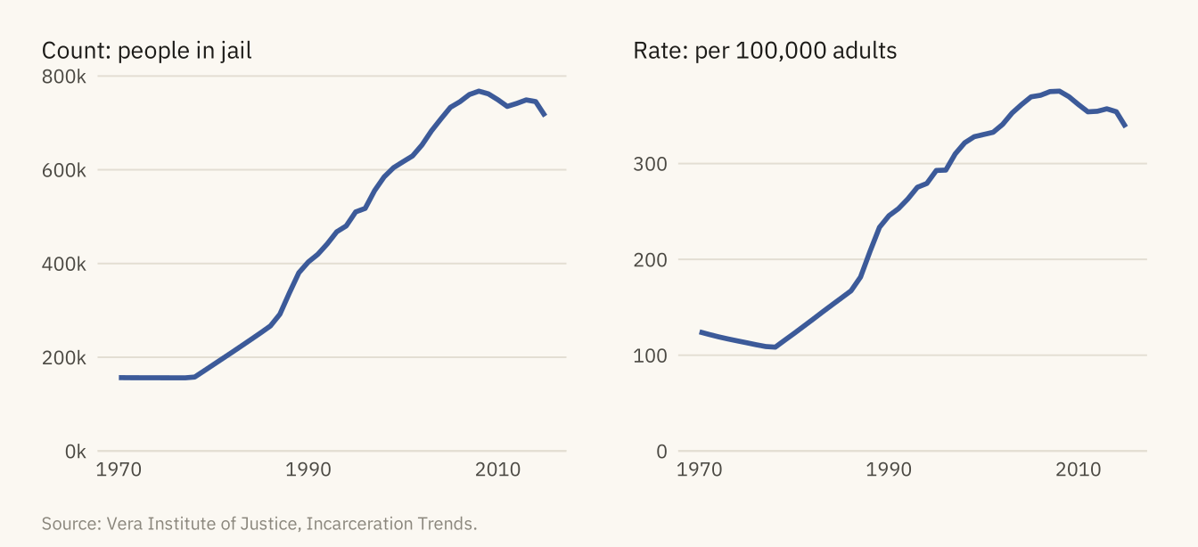
Figure 7.3
Jail and state prison populations, 1983 to 2013, on one scale. Prison grew faster and further. Both series peaked in 2008. Jail has stayed below its peak since. Prison held level through 2010 and then came down slowly. Both series end in 2013 because county coverage drops after that, as the next figure shows. Source: Vera Institute of Justice, Incarceration Trends.
Code
two <- bind_rows(jail |> filter(year >= 1983, year <= 2013) |> transmute(year, series = "County jails", n = jail),
                 prison |> transmute(year, series = "State prisons", n = prison))
ends <- two |> group_by(series) |> slice_max(year, n = 1)
ggplot(two, aes(year, n, color = series)) +
  geom_line(linewidth = 1.1) +
  mv_label_end(ends, aes(label = series, color = series), nudge_x = 0.4) +
  scale_color_manual(values = c(`County jails` = mv_accent(), `State prisons` = mv_ink$ink), guide = "none") +
  scale_x_continuous(breaks = seq(1985, 2015, 5), limits = c(1983, 2021), expand = expansion(mult = 0.01)) +
  scale_y_continuous(labels = label_comma(scale = 1e-6, accuracy = 0.1, suffix = " M"), limits = c(0, 1.4e6), expand = expansion(0)) +
  labs(title = "Jail and state prison populations, 1983 to 2013",
       subtitle = "People held on a single day, both series on one scale",
       x = NULL, y = NULL, caption = mv_source(src)) +
  theme_mv()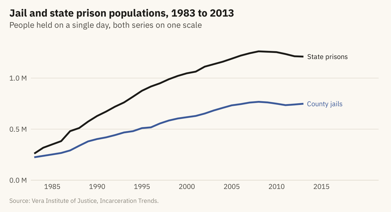
Figure 7.4
Jail population, prison population, and adult population, each as a share of its 1983 value. By 2008, the prison population was 4.8 times its 1983 level and the jail population 3.4 times, while the adult population grew by a third. Source: Vera Institute of Justice, Incarceration Trends.
Code
idx <- nat |> filter(year >= 1983, year <= 2013) |>
  transmute(year, `State prisons` = prison / prison[year == 1983] * 100,
            `County jails` = jail / jail[year == 1983] * 100,
            `Adults aged 15 to 64` = pop_15to64 / pop_15to64[year == 1983] * 100) |>
  pivot_longer(-year, names_to = "series", values_to = "index")
iend <- idx |> filter(year == 2013)
ggplot(idx, aes(year, index, color = series)) +
  geom_hline(yintercept = 100, color = mv_ink$mute, linewidth = 0.4) +
  geom_line(linewidth = 1) +
  mv_label_end(iend, aes(label = series, color = series), nudge_x = 0.4) +
  scale_color_manual(values = c(`State prisons` = mv_ink$ink, `County jails` = mv_accent(), `Adults aged 15 to 64` = mv_ink$mute), guide = "none") +
  scale_x_continuous(breaks = seq(1985, 2015, 5), limits = c(1983, 2024), expand = expansion(mult = 0.01)) +
  scale_y_continuous(limits = c(0, 520), expand = expansion(0)) +
  labs(title = "Jail, prison, and adult population, indexed to 1983",
       subtitle = "Each series as a share of its 1983 level (1983 = 100)",
       x = NULL, y = NULL, caption = mv_source(src)) +
  theme_mv()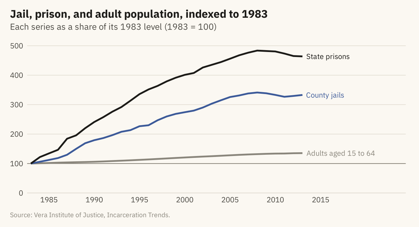
Figure 7.5
The summed prison count through 2015 (top) and the number of counties reporting each year (bottom). The drop after 2013 comes from counties missing from the data, not from a fall in the prison population. The series is reliable only for the years with full coverage, and the coverage should be shown on the chart or stated in its caption. Source: Vera Institute of Justice, Incarceration Trends.
Code
cov <- nat |> filter(year >= 1983)
top <- ggplot(cov, aes(year, prison)) +
  annotate("rect", xmin = 2013.5, xmax = 2015.5, ymin = 0, ymax = Inf, fill = mv_ink$mute, alpha = 0.25) +
  geom_line(color = mv_ink$ink, linewidth = 1) +
  annotate("text", x = 2013.3, y = 1.42e6, label = "Looks like a fall", hjust = 1, vjust = 1, size = 3, family = mv_font(), color = mv_ink$ink2) +
  scale_x_continuous(breaks = seq(1985, 2015, 5)) +
  scale_y_continuous(labels = label_comma(scale = 1e-6, accuracy = 0.1, suffix = " M"), limits = c(0, 1.5e6), expand = expansion(0)) +
  labs(x = NULL, y = NULL, title = "Summed prison population") + theme_mv(base_size = 10) + plain_title
bot <- ggplot(cov, aes(year, prison_reported)) +
  annotate("rect", xmin = 2013.5, xmax = 2015.5, ymin = 0, ymax = Inf, fill = mv_ink$mute, alpha = 0.25) +
  geom_col(fill = mv_accent(), width = 0.8) +
  annotate("text", x = 2013.3, y = 3250, label = "Counties stop reporting", hjust = 1, vjust = 1, size = 3, family = mv_font(), color = mv_ink$ink2) +
  scale_x_continuous(breaks = seq(1985, 2015, 5)) +
  scale_y_continuous(labels = label_comma(), breaks = c(0, 1000, 2000, 3000), limits = c(0, 3300), expand = expansion(0)) +
  labs(x = NULL, y = NULL, title = "Counties reporting a prison count") + theme_mv(base_size = 10) + plain_title
(top / bot) + plot_layout(heights = c(1.4, 1)) + plot_annotation(caption = mv_source(src), theme = cap_theme)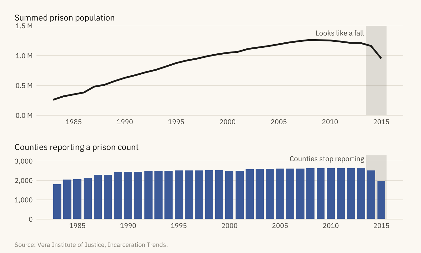
Figure 7.6
Jail population per 100,000 adults aged 15 to 64 in each state and DC, 1990 to 2015, on a shared vertical scale and sorted by the 2015 rate. Louisiana is far above the rest, at about 960 in 2015. Kentucky, Tennessee, Mississippi, Georgia, and New Mexico form the next group, between 600 and 725. Six states run unified systems with no county jails and are omitted. Source: Vera Institute of Justice, Incarceration Trends.
Code
sts <- st |> filter(year >= 1990, year <= 2015) |>
  group_by(state) |> filter(all(jail_rate > 0)) |> ungroup() |>
  mutate(state = fct_reorder(state, jail_rate, .fun = \(x) -x[length(x)]))
ggplot(sts, aes(year, jail_rate)) +
  geom_area(fill = mv_accent(), alpha = 0.2) +
  geom_line(color = mv_accent(), linewidth = 0.6) +
  facet_wrap(~ state, ncol = 9) +
  scale_x_continuous(breaks = c(1990, 2015), labels = c("'90", "'15")) +
  scale_y_continuous(breaks = c(0, 500, 1000), expand = expansion(mult = c(0, 0.05))) +
  labs(title = "Jail rate by state, 1990 to 2015",
       subtitle = "Jail population per 100,000 adults, 1990 to 2015, sorted by the 2015 rate",
       x = NULL, y = NULL, caption = mv_source(src, "AK, CT, DE, HI, RI, and VT omitted")) +
  theme_mv(base_size = 9, grid = "none") +
  theme(strip.text = element_text(size = rel(0.85), margin = margin(b = 1)),
        axis.text = element_text(size = rel(0.75)), panel.spacing.y = unit(0.5, "lines"),
        panel.spacing.x = unit(1.4, "lines"))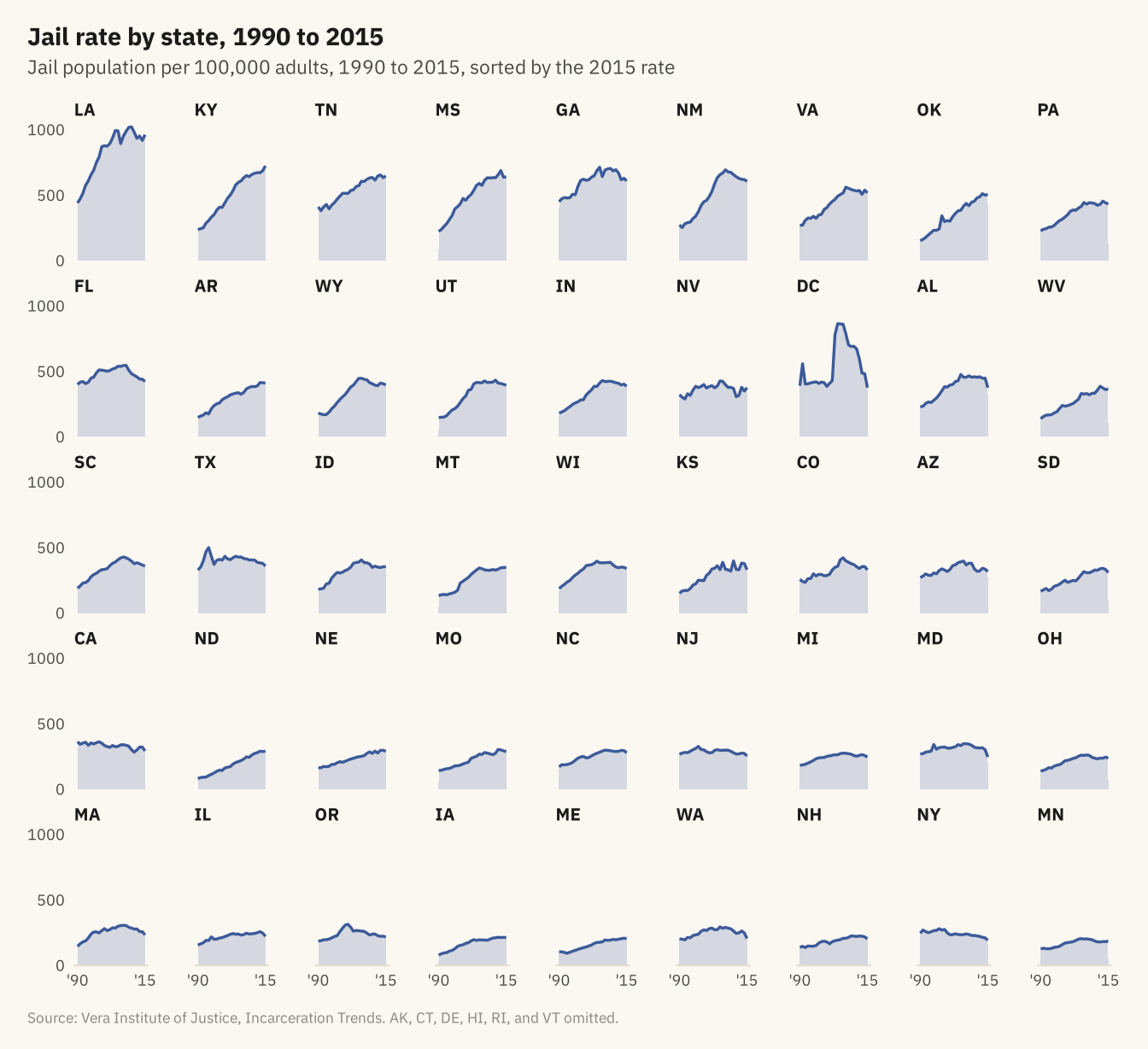
Figure 7.7
The jail rate against the prison rate, one point per year from 1983 to 2013, connected in order. Both rose together through 2008, when the path turns. From 2008 to 2013 the jail rate fell from 376 to 357 and the prison rate from 617 to 577, so the path doubles back down and to the left along the way it came. Source: Vera Institute of Justice, Incarceration Trends.
Code
cs <- nat |> filter(year >= 1983, year <= 2013)
marks <- cs |> filter(year %in% c(1983, 1990, 2000, 2008, 2013)) |>
  mutate(dx = c(8, 8, -8, 0, 8), dy = c(-22, -22, 28, 30, -30), hj = c(0, 0, 1, 0.5, 0))
ggplot(cs, aes(jail_rate, prison_rate)) +
  geom_path(color = mv_accent(), linewidth = 0.9, lineend = "round") +
  geom_point(data = marks, color = mv_accent(), size = 2.6) +
  geom_text(data = marks, aes(x = jail_rate + dx, y = prison_rate + dy, label = year, hjust = hj),
            size = 3, family = mv_font(), color = mv_ink$ink2) +
  scale_x_continuous(limits = c(0, NA), expand = expansion(mult = c(0, 0.05))) +
  scale_y_continuous(limits = c(0, NA), expand = expansion(mult = c(0, 0.08))) +
  labs(title = "Jail rate and prison rate, 1983 to 2013",
       subtitle = "Jail and prison population per 100,000 adults, 1983 to 2013, connected by year",
       x = "Jail rate", y = "Prison rate", caption = mv_source(src)) +
  theme_mv(grid = "y") +
  theme(panel.grid.major.x = element_line(color = mv_ink$grid, linewidth = 0.35))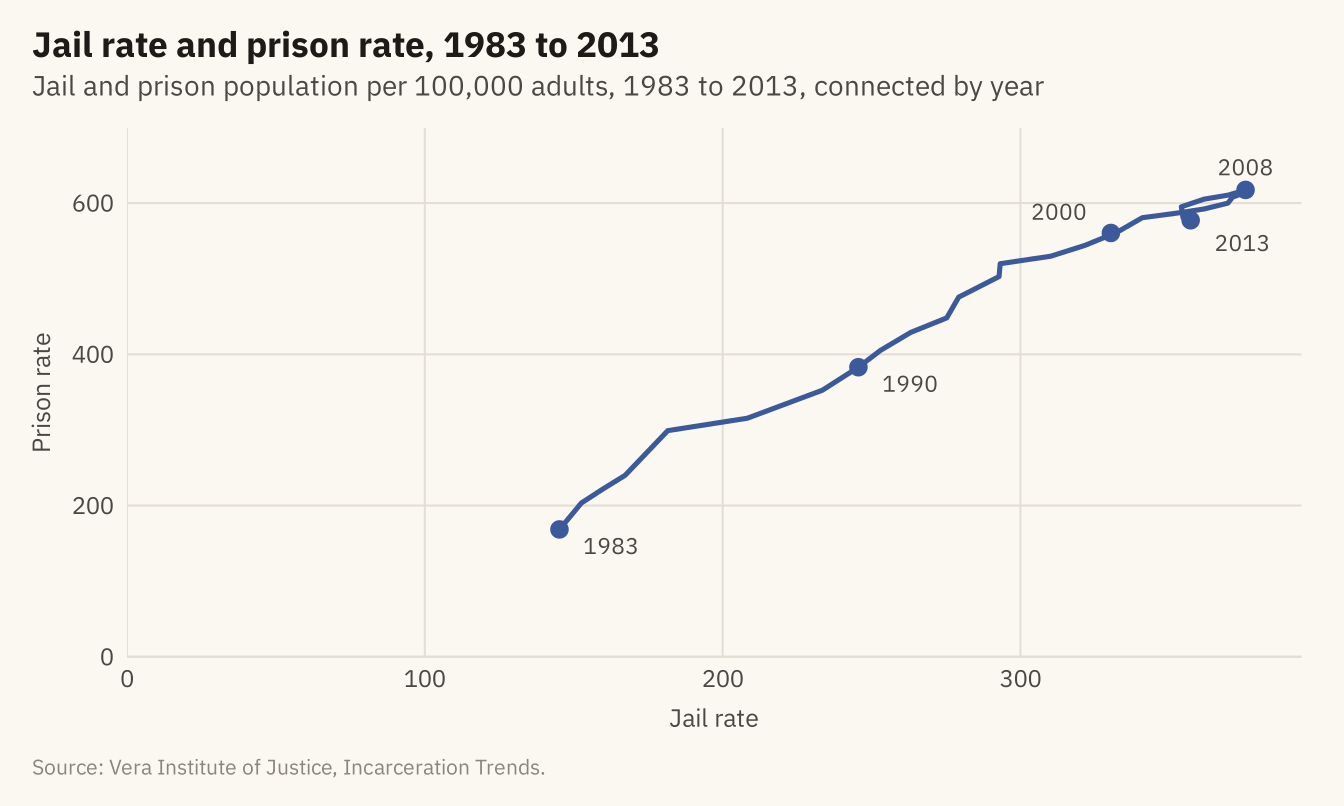
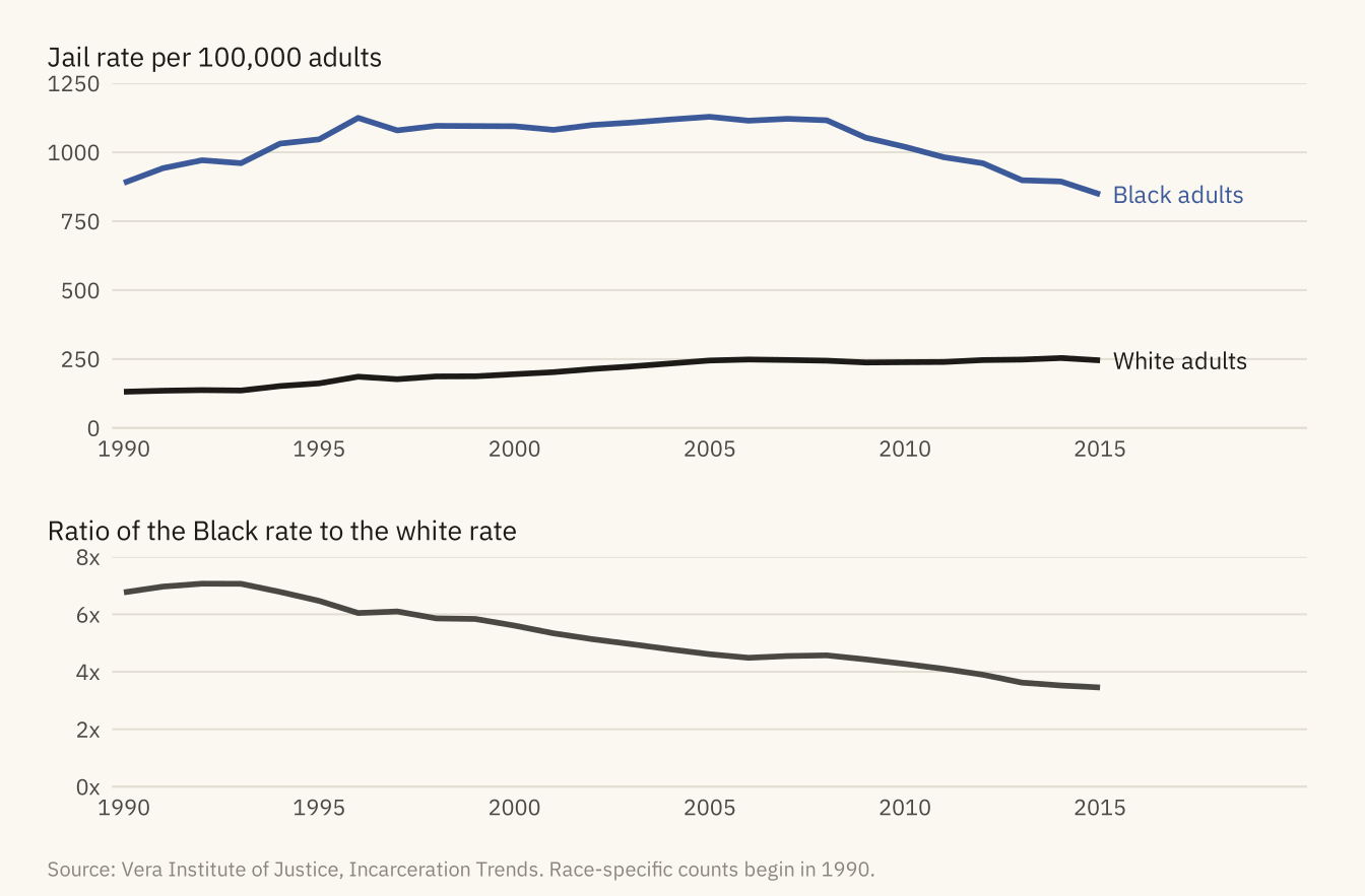
Figure 7.8
Jail population per 100,000 adults aged 15 to 64, Black and white, 1990 to 2015 (top), and the ratio between them (bottom). The white rate rose from 131 to about 245 by 2005 and then held there. The Black rate held near 1,100 from 1996 to 2008 and then fell to 847. The ratio fell from near seven to under four. Source: Vera Institute of Justice, Incarceration Trends. Race-specific counts begin in 1990.
Code
race <- nat |> filter(year >= 1990) |>
  transmute(year, Black = 1e5 * jail_black / pop_black, White = 1e5 * jail_white / pop_white, ratio = Black / White)
rl <- race |> pivot_longer(c(Black, White), names_to = "group", values_to = "rate")
rend <- rl |> filter(year == 2015)
p1 <- ggplot(rl, aes(year, rate, color = group)) +
  geom_line(linewidth = 1) +
  mv_label_end(rend, aes(label = paste(group, "adults"), color = group), nudge_x = 0.3) +
  scale_color_manual(values = c(Black = mv_accent(), White = mv_ink$ink), guide = "none") +
  scale_x_continuous(breaks = seq(1990, 2015, 5), limits = c(1990, 2020), expand = expansion(mult = 0.01)) +
  scale_y_continuous(limits = c(0, 1250), expand = expansion(0)) +
  labs(x = NULL, y = NULL, title = "Jail rate per 100,000 adults") + theme_mv(base_size = 10) + plain_title
p2 <- ggplot(race, aes(year, ratio)) +
  geom_line(color = mv_ink$ink2, linewidth = 1) +
  scale_x_continuous(breaks = seq(1990, 2015, 5), limits = c(1990, 2020), expand = expansion(mult = 0.01)) +
  scale_y_continuous(limits = c(0, 8), breaks = c(0, 2, 4, 6, 8), labels = \(x) paste0(x, "x"), expand = expansion(0)) +
  labs(x = NULL, y = NULL, title = "Ratio of the Black rate to the white rate") + theme_mv(base_size = 10) + plain_title
(p1 / p2) + plot_layout(heights = c(1.5, 1)) + plot_annotation(caption = mv_source(src, "Race-specific counts begin in 1990"), theme = cap_theme)