# Where the data and the theme live. The defaults load from the companion
# site. Set MV_DATA and MV_THEME to local paths to work offline.
mv_data  <- Sys.getenv("MV_DATA",  "https://viz.marginoferrormedia.com/data")
mv_theme <- Sys.getenv("MV_THEME", "https://viz.marginoferrormedia.com/figures/mv-theme.R")Chapter 6: Relationship
The code behind every figure in Chapter 6 of Make It Visible, in the order the chapter draws them. Run the first chunk, then any figure. Each chunk stands on its own once the setup chunk has run.
Setup
Loads the theme, the packages, and the chapter’s data.
Code
source(mv_theme)
mv_set_chapter(6)
suppressPackageStartupMessages({ library(tidyverse); library(ggrepel); library(patchwork) })
m <- read_csv(file.path(mv_data, "ch06-college-majors.csv"), show_col_types = FALSE)
cap_theme <- theme(plot.caption = element_text(size = 7.5, hjust = 0, color = mv_ink$mute, family = mv_font()),
                   plot.background = element_rect(fill = mv_ink$canvas, color = NA))
plain_title <- theme(plot.title = element_text(size = rel(1), face = "plain"))
src <- "American Community Survey 2010 to 2012, via FiveThirtyEight"
r_all <- cor(m$share_women, m$median)
Figure 6.1
Median earnings of recent graduates against the share of women among graduates, one point per major. The relationship is negative and loose. The correlation is -0.62. Source: American Community Survey 2010 to 2012, via FiveThirtyEight.
Code
ggplot(m, aes(share_women, median)) +
  geom_point(color = mv_accent(), size = 2, alpha = 0.7) +
  scale_x_continuous(labels = label_percent()) +
  scale_y_continuous(labels = label_dollar(scale = 1e-3, suffix = "k"), limits = c(0, NA), expand = expansion(mult = c(0, 0.05))) +
  labs(title = "Median earnings of recent graduates by share of women in the major",
       subtitle = "172 majors, one point per major. Median earnings in dollars.",
       x = "Share of graduates who are women", y = "Median earnings",
       caption = mv_source(src)) +
  theme_mv(grid = "y") +
  theme(panel.grid.major.x = element_line(color = mv_ink$grid, linewidth = 0.35))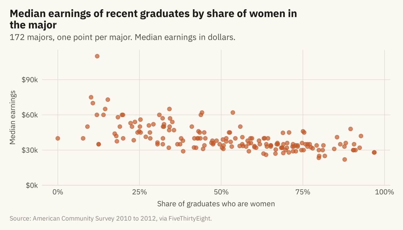
Figure 6.2
The same points with a straight-line fit (solid) and a local smoother (dashed). The slope of the line means that a major with ten points more women pays about $3,100 less. The smoother follows the line across most of the range and flattens at the right. The band around the line shows the uncertainty in the line, not the spread of the points. Source: American Community Survey 2010 to 2012, via FiveThirtyEight.
Code
slope <- coef(lm(median ~ share_women, m))[2]
ggplot(m, aes(share_women, median)) +
  geom_point(color = mv_accent(), size = 1.8, alpha = 0.5) +
  geom_smooth(method = "loess", se = FALSE, color = mv_ink$ink, linewidth = 0.7, linetype = "22", formula = y ~ x, span = 0.9) +
  geom_smooth(method = "lm", color = mv_ink$ink, fill = mv_ink$ink, alpha = 0.22, linewidth = 0.9, formula = y ~ x) +
  annotate("text", x = 0.88, y = 54000, label = paste0("Each 10 points more women:\n", label_dollar()(round(-slope / 10, -2)), " less"),
           hjust = 1, size = 3, family = mv_font(), color = mv_ink$ink, lineheight = 0.95) +
  scale_x_continuous(labels = label_percent()) +
  scale_y_continuous(labels = label_dollar(scale = 1e-3, suffix = "k"), limits = c(0, NA), expand = expansion(mult = c(0, 0.05))) +
  labs(title = "Median earnings by share of women, with a linear fit and a local smoother",
       subtitle = "172 majors. Solid line: linear fit with its confidence band. Dashed line: local smoother.",
       x = "Share of graduates who are women", y = "Median earnings", caption = mv_source(src)) +
  theme_mv(grid = "y") +
  theme(panel.grid.major.x = element_line(color = mv_ink$grid, linewidth = 0.35))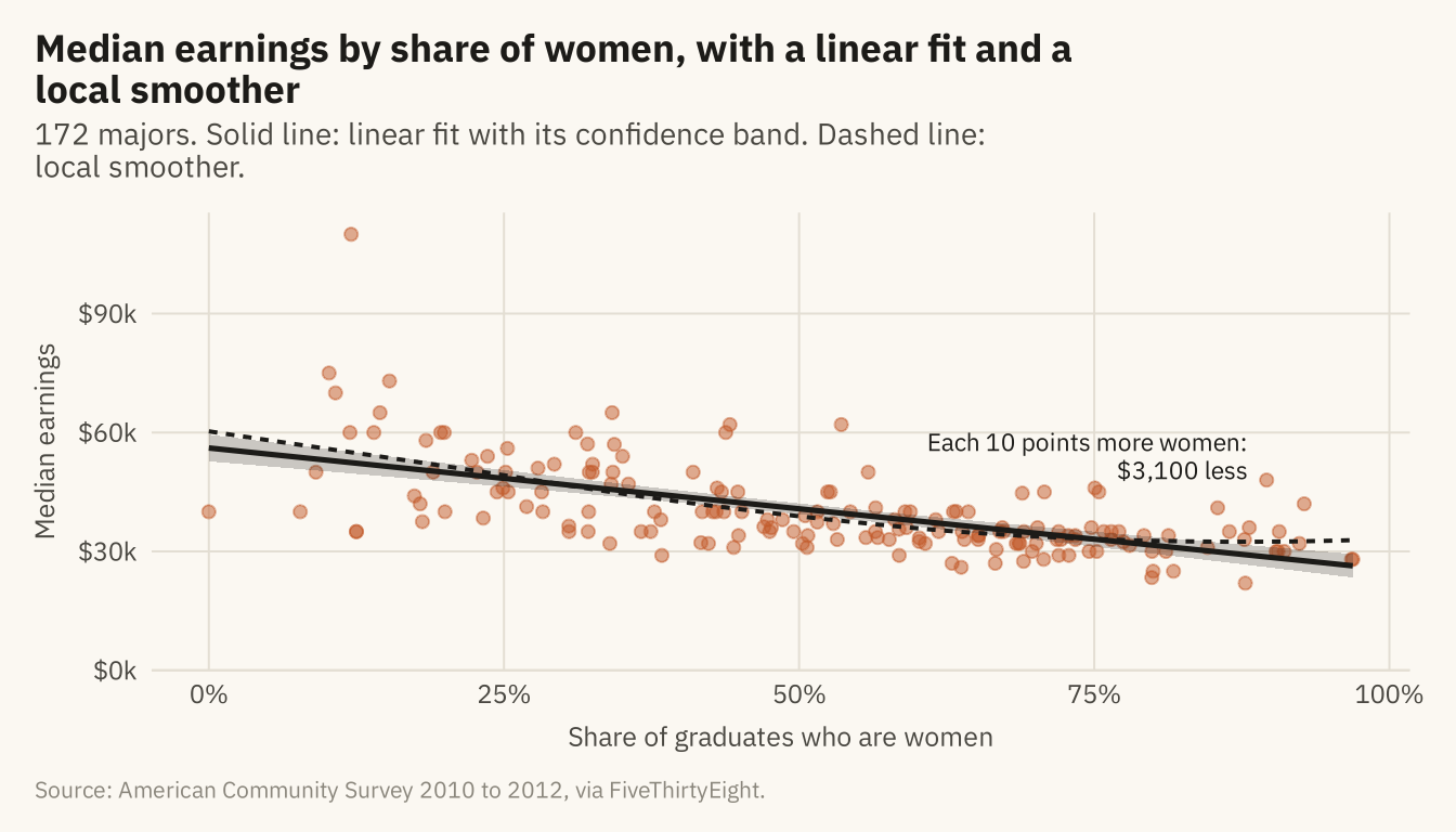
Figure 6.3
The same relationship with each major sized by its number of graduates. Named: the three highest and two lowest medians, and the seven majors with more than 200,000 graduates. Petroleum engineering, with 2,300 graduates, is alone at the top. Psychology, with 393,000, is among the many majors at the lower right. The three largest majors are psychology, business administration, and biology. Source: American Community Survey 2010 to 2012, via FiveThirtyEight.
Code
named <- m |> filter(median >= 73000 | median <= 23500 | graduates >= 200000) |>
  mutate(major = str_replace(major, "Business Management and Administration", "Business Admin."),
         ny = case_when(major %in% c("General Business", "Marketing and Marketing Research") ~ 14000,
                        major %in% c("Business Admin.", "Biology", "Communications") ~ -14000,
                        major == "Psychology" ~ -16000,
                        major == "Counseling Psychology" ~ -12000,
                        major == "Library Science" ~ -9000,
                        major == "Nursing" ~ 12000,
                        TRUE ~ 0),
         nx = case_when(major == "General Business" ~ -0.12, major == "Business Admin." ~ -0.1,
                        major == "Marketing and Marketing Research" ~ 0.08,
                        major == "Biology" ~ -0.08, major == "Communications" ~ 0.04,
                        major == "Psychology" ~ -0.12, major == "Counseling Psychology" ~ -0.02,
                        major == "Library Science" ~ 0.03, major == "Nursing" ~ -0.06,
                        TRUE ~ 0))
ggplot(m, aes(share_women, median)) +
  geom_point(aes(size = graduates), color = mv_accent(), alpha = 0.45) +
  geom_point(data = named, aes(size = graduates), color = mv_ink$ink, shape = 21, stroke = 0.5, fill = NA) +
  geom_text_repel(data = named, aes(label = major), size = 2.6, family = mv_font(), color = mv_ink$ink,
                  nudge_x = named$nx, nudge_y = named$ny,
                  min.segment.length = 0, segment.color = mv_ink$mute, segment.size = 0.3,
                  box.padding = 0.45, point.padding = 0.3, max.overlaps = 30, seed = 6) +
  scale_size_area(max_size = 14, guide = "none") +
  scale_x_continuous(labels = label_percent()) +
  scale_y_continuous(labels = label_dollar(scale = 1e-3, suffix = "k"), limits = c(0, NA), expand = expansion(mult = c(0, 0.05))) +
  labs(title = "Median earnings by share of women, point size by number of graduates",
       subtitle = "172 majors. Point area is proportional to the number of graduates. Outliers named.",
       x = "Share of graduates who are women", y = "Median earnings", caption = mv_source(src)) +
  theme_mv(grid = "y") +
  theme(panel.grid.major.x = element_line(color = mv_ink$grid, linewidth = 0.35))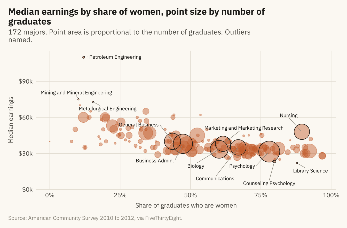
Figure 6.4
Median earnings by share of women within each of eight fields, with a fitted line per field, all on the same axes. The slope is steep within engineering and business, shallow within education and humanities, and flat within computing, biology, and health. Part of the overall pattern is between fields and part is within them. Source: American Community Survey 2010 to 2012, via FiveThirtyEight.
Code
cats <- m |> count(category) |> filter(n >= 10) |> pull(category)
fm <- m |> filter(category %in% cats) |>
  mutate(category = str_replace(category, " & ", " and "),
         category = fct_reorder(category, median, .fun = stats::median, .desc = TRUE))
ggplot(fm, aes(share_women, median)) +
  geom_point(data = select(m, -category), color = mv_ink$grid, size = 0.9) +
  geom_point(color = mv_accent(), size = 1.6, alpha = 0.8) +
  geom_smooth(method = "lm", se = FALSE, color = mv_ink$ink, linewidth = 0.6, formula = y ~ x) +
  facet_wrap(~ category, ncol = 4, labeller = label_wrap_gen(22)) +
  scale_x_continuous(labels = label_percent(), breaks = c(0, 0.5, 1)) +
  scale_y_continuous(labels = label_dollar(scale = 1e-3, suffix = "k"), breaks = c(25000, 50000, 75000, 100000)) +
  labs(title = "Median earnings by share of women within eight fields",
       subtitle = "Each panel is one field, in color, against all 172 majors in grey",
       x = "Share of graduates who are women", y = "Median earnings", caption = mv_source(src)) +
  theme_mv(base_size = 10) +
  theme(strip.text = element_text(size = rel(0.8)))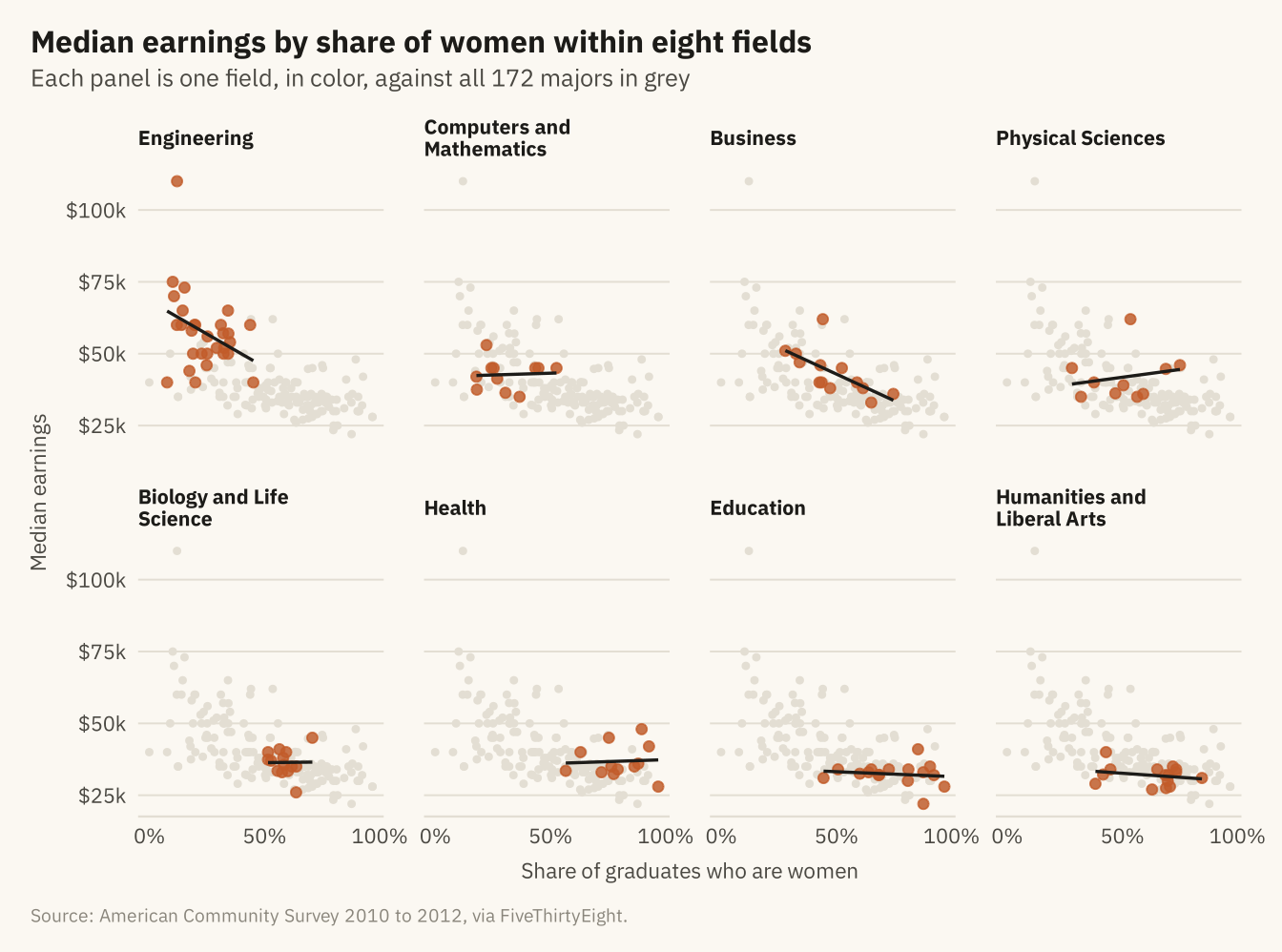
Figure 6.5
Correlations among five measures across 172 majors. Earnings rise with the share of graduates in jobs that need a degree and fall with the share of women. Unemployment is only weakly correlated with the other measures. A correlation grid shows which measures move together, and nothing about why. Source: American Community Survey 2010 to 2012, via FiveThirtyEight.
Code
vars <- m |> transmute(`Median earnings` = median, `Share women` = share_women,
                       `Unemployment rate` = unemployment_rate, `Share in degree jobs` = share_college_jobs,
                       `Number of graduates` = log10(graduates))
cm <- cor(vars, use = "pairwise.complete.obs") |> as.data.frame() |> rownames_to_column("a") |>
  pivot_longer(-a, names_to = "b", values_to = "r") |>
  mutate(a = factor(a, levels = names(vars)), b = factor(b, levels = rev(names(vars))))
ggplot(cm, aes(a, b, fill = r)) +
  geom_tile(color = mv_ink$canvas, linewidth = 1) +
  geom_text(aes(label = sprintf("%.2f", r), color = abs(r) > 0.5), size = 3, family = mv_font()) +
  scale_color_manual(values = c(`TRUE` = mv_ink$canvas, `FALSE` = mv_ink$ink), guide = "none") +
  scale_fill_gradient2(low = "#3C5A99", mid = "#F2EDE2", high = mv_accent(), limits = c(-1, 1), guide = "none") +
  scale_x_discrete(labels = label_wrap(12), position = "top") +
  labs(title = "Correlations among five measures, 172 majors", x = NULL, y = NULL, caption = mv_source(src, "Graduates on a log scale")) +
  theme_mv(grid = "none") +
  theme(axis.text.x = element_text(size = rel(0.8), lineheight = 0.9), axis.line.x = element_blank())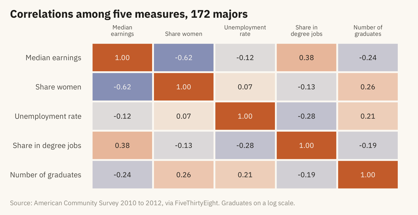
Figure 6.6
The middle half of earnings (25th to 75th percentile) for the twenty largest majors, sorted by median. The ranges overlap heavily. A nursing graduate at the 75th percentile earns more than a computer science graduate at the 25th. Source: American Community Survey 2010 to 2012, via FiveThirtyEight.
Code
big <- m |> slice_max(graduates, n = 20) |>
  mutate(major = str_replace(major, "Business Management and Administration", "Business Admin."),
         major = fct_reorder(major, median))
ggplot(big) +
  geom_segment(aes(x = p25, xend = p75, y = major, yend = major), color = mv_accent(), linewidth = 3, alpha = 0.35, lineend = "round") +
  geom_point(aes(median, major), color = mv_accent(), size = 2.4) +
  scale_x_continuous(labels = label_dollar(scale = 1e-3, suffix = "k"), limits = c(0, NA), expand = expansion(mult = c(0, 0.04))) +
  labs(title = "Median and middle half of earnings, twenty largest majors",
       subtitle = "Dot: median. Bar: 25th to 75th percentile. Earnings of recent graduates in dollars.",
       x = NULL, y = NULL, caption = mv_source(src)) +
  theme_mv(grid = "x")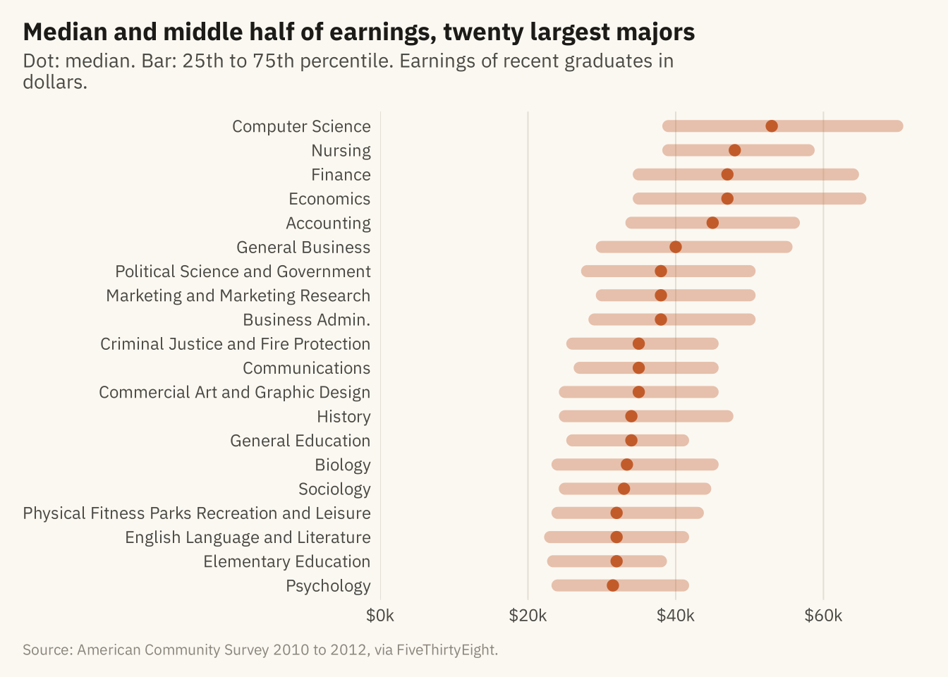
Figure 6.7
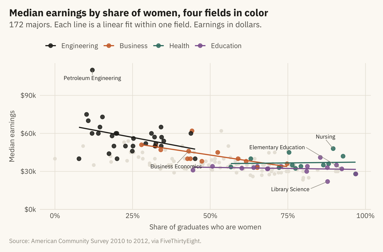
Median earnings by share of women, with four fields in color and the rest in grey. Engineering is at the upper left and education at the lower right. Part of the overall slope is the distance between them. Within business the slope is steep. Within health it is flat, and nursing is the main reason. Source: American Community Survey 2010 to 2012, via FiveThirtyEight.
Code
four <- c("Engineering", "Business", "Health", "Education")
fin <- m |> mutate(grp = if_else(category %in% four, category, "Other"),
                   grp = factor(grp, levels = c(four, "Other")))
cols <- c(Engineering = mv_ink$ink, Business = mv_accent(), Health = "#2E6B5E", Education = "#7A4E8C", Other = mv_ink$grid)
labs_pts <- m |> filter(major %in% c("Petroleum Engineering", "Nursing", "Elementary Education", "Business Economics",
                                     "Library Science")) |>
  mutate(ny = case_when(major == "Elementary Education" ~ 18000, major == "Business Economics" ~ -12000,
                        major == "Library Science" ~ -6000, major == "Nursing" ~ 9000, TRUE ~ 0),
         nx = case_when(major == "Elementary Education" ~ -0.2, major == "Business Economics" ~ -0.04,
                        major == "Library Science" ~ -0.12, major == "Nursing" ~ -0.03, TRUE ~ 0))
ggplot(fin, aes(share_women, median, color = grp)) +
  geom_point(data = filter(fin, grp == "Other"), size = 1.6) +
  geom_point(data = filter(fin, grp != "Other"), size = 2.2, alpha = 0.85) +
  geom_smooth(data = filter(fin, grp != "Other"), method = "lm", se = FALSE, linewidth = 0.7, formula = y ~ x) +
  geom_text_repel(data = labs_pts, aes(label = major), color = mv_ink$ink, size = 2.6, family = mv_font(),
                  nudge_x = labs_pts$nx, nudge_y = labs_pts$ny,
                  min.segment.length = 0, segment.color = mv_ink$mute, segment.size = 0.3, box.padding = 0.5, seed = 3) +
  scale_color_manual(values = cols, breaks = four, name = NULL) +
  scale_x_continuous(labels = label_percent()) +
  scale_y_continuous(labels = label_dollar(scale = 1e-3, suffix = "k"), limits = c(0, NA), expand = expansion(mult = c(0, 0.05))) +
  labs(title = "Median earnings by share of women, four fields in color",
       subtitle = "172 majors. Each line is a linear fit within one field. Earnings in dollars.",
       x = "Share of graduates who are women", y = "Median earnings", caption = mv_source(src)) +
  theme_mv(grid = "y") +
  theme(panel.grid.major.x = element_line(color = mv_ink$grid, linewidth = 0.35))