# Where the data and the theme live. The defaults load from the companion
# site. Set MV_DATA and MV_THEME to local paths to work offline.
mv_data  <- Sys.getenv("MV_DATA",  "https://viz.marginoferrormedia.com/data")
mv_theme <- Sys.getenv("MV_THEME", "https://viz.marginoferrormedia.com/figures/mv-theme.R")Chapter 5: Distribution
The code behind every figure in Chapter 5 of Make It Visible, in the order the chapter draws them. Run the first chunk, then any figure. Each chunk stands on its own once the setup chunk has run.
Setup
Loads the theme, the packages, and the chapter’s data.
Code
source(mv_theme)
mv_set_chapter(5)
suppressPackageStartupMessages({ library(tidyverse); library(ggrepel); library(patchwork); library(ggridges) })
d <- read_csv(file.path(mv_data, "ch05-school-districts.csv"), show_col_types = FALSE) |>
  mutate(locale = factor(locale, levels = c("City", "Suburb", "Town", "Rural")))
d17 <- filter(d, year == 2017)
cap_theme <- theme(plot.caption = element_text(size = 7.5, hjust = 0, color = mv_ink$mute, family = mv_font()),
                   plot.background = element_rect(fill = mv_ink$canvas, color = NA))
plain_title <- theme(plot.title = element_text(size = rel(1), face = "plain"))
src <- "NCES Common Core of Data, via the Washington Post"
w_mean <- with(d17, sum(white * enrollment) / sum(enrollment))
Figure 5.1
Share of white students in each of 12,399 school districts, 2016-17, in bins of 2.5 points. Most districts are near 90 percent, and a long tail runs toward zero. The district mean (70) and the student-weighted mean (49) are marked. Neither falls where most districts are. Source: NCES Common Core of Data, via the Washington Post.
Code
ggplot(d17, aes(white)) +
  geom_histogram(binwidth = 2.5, boundary = 0, fill = mv_accent(), color = mv_ink$canvas, linewidth = 0.3) +
  geom_vline(xintercept = mean(d17$white), color = mv_ink$ink, linewidth = 0.6) +
  geom_vline(xintercept = w_mean, color = mv_ink$ink, linewidth = 0.6, linetype = "22") +
  annotate("text", x = mean(d17$white) + 1.5, y = 1550, label = "Mean district: 70%", hjust = 0,
           size = 2.9, family = mv_font(), color = mv_ink$ink) +
  annotate("text", x = w_mean - 1.5, y = 1350, label = paste0("Mean student's district: ", round(w_mean), "%"),
           hjust = 1, size = 2.9, family = mv_font(), color = mv_ink$ink) +
  scale_x_continuous(labels = label_percent(scale = 1), expand = expansion(0)) +
  scale_y_continuous(expand = expansion(mult = c(0, 0.05))) +
  labs(title = "Share of white students in 12,399 school districts, 2016-17",
       subtitle = "Number of districts by share of white students. Lines mark the two means.",
       x = NULL, y = NULL, caption = mv_source(src)) +
  theme_mv()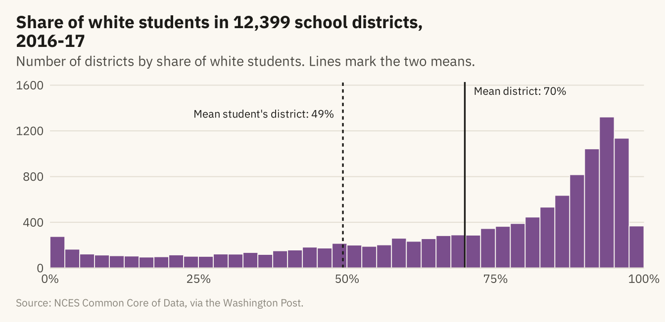
Figure 5.2
The same distribution with bins of 20, 5, and 1 percentage point. The wide bins leave out the shape. The narrow bins are jagged, and neighboring bars differ by chance. The middle panel shows the shape with the least noise. Source: NCES Common Core of Data, via the Washington Post.
Code
bins <- function(bw, title) {
  ggplot(d17, aes(white)) +
    geom_histogram(binwidth = bw, boundary = 0, fill = mv_accent(), color = mv_ink$canvas, linewidth = 0.2) +
    scale_x_continuous(labels = label_percent(scale = 1), breaks = c(0, 50, 100), expand = expansion(0)) +
    scale_y_continuous(expand = expansion(mult = c(0, 0.05))) +
    labs(x = NULL, y = NULL, title = title) + theme_mv(base_size = 10) + plain_title +
    theme(axis.text.y = element_blank())
}
bins(20, "Bins of 20 points") + bins(5, "Bins of 5 points") + bins(1, "Bins of 1 point") +
  plot_annotation(caption = mv_source(src), theme = cap_theme)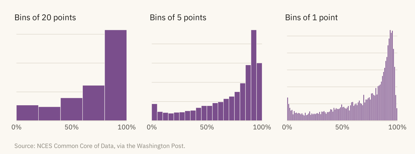
Figure 5.3
District enrollment, 2016-17. Left, on a linear axis, nearly every district falls in the first bar, and the axis extends past 900,000 because of New York City. Right, on a log axis, the distribution is bell-shaped and centered near 1,200 students. The largest districts form a thin tail on the right. Source: NCES Common Core of Data, via the Washington Post.
Code
lin <- ggplot(d17, aes(enrollment)) +
  geom_histogram(bins = 60, fill = mv_accent(), color = mv_ink$canvas, linewidth = 0.2) +
  scale_x_continuous(labels = label_comma(), expand = expansion(0)) +
  scale_y_continuous(expand = expansion(mult = c(0, 0.05))) +
  labs(x = NULL, y = NULL, title = "Linear axis") + theme_mv(base_size = 10) + plain_title
lg <- ggplot(d17, aes(enrollment)) +
  geom_histogram(bins = 40, fill = mv_accent(), color = mv_ink$canvas, linewidth = 0.2) +
  scale_x_log10(labels = c("100", "1k", "10k", "100k", "1M"), breaks = c(100, 1000, 10000, 100000, 1e6), expand = expansion(0)) +
  scale_y_continuous(expand = expansion(mult = c(0, 0.05))) +
  labs(x = NULL, y = NULL, title = "Log axis") + theme_mv(base_size = 10) + plain_title
lin + lg + plot_annotation(caption = mv_source(src), theme = cap_theme)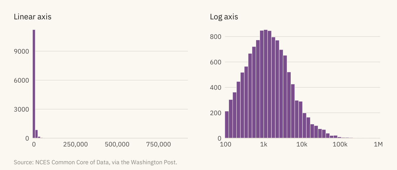
Figure 5.4
Share of white students by district locale, 2016-17, drawn three ways. The box plot shows the median and middle half. The violin shows the full shape, including the pile-up of rural districts near 100 percent. The dots show every district and how many there are in each group. Source: NCES Common Core of Data, via the Washington Post.
Code
set.seed(5)
outs <- d17 |> group_by(locale) |>
  filter(white < quantile(white, 0.25) - 1.5 * IQR(white) | white > quantile(white, 0.75) + 1.5 * IQR(white)) |>
  ungroup()
bx <- ggplot(d17, aes(white, fct_rev(locale))) +
  geom_boxplot(fill = mv_accent(), color = mv_ink$ink, alpha = 0.6, width = 0.55, outlier.shape = NA) +
  geom_point(data = outs, position = position_jitter(height = 0.14, width = 0, seed = 5),
             size = 0.35, alpha = 0.3, color = mv_ink$ink) +
  scale_x_continuous(labels = label_percent(scale = 1), breaks = c(0, 50, 100)) +
  labs(x = NULL, y = NULL, title = "Box: median and\nmiddle half") + theme_mv(base_size = 10, grid = "x") + plain_title
vn <- ggplot(d17, aes(white, fct_rev(locale))) +
  geom_violin(fill = mv_accent(), color = NA, alpha = 0.7, scale = "width", width = 0.8) +
  stat_summary(fun = median, geom = "point", shape = 124, size = 4, color = mv_ink$ink) +
  scale_x_continuous(labels = label_percent(scale = 1), breaks = c(0, 50, 100)) +
  labs(x = NULL, y = NULL, title = "Violin: density\nof each group") + theme_mv(base_size = 10, grid = "x") + plain_title +
  theme(axis.text.y = element_blank())
dt <- ggplot(d17, aes(white, fct_rev(locale))) +
  geom_jitter(height = 0.3, width = 0, size = 0.4, alpha = 0.25, color = mv_accent()) +
  scale_x_continuous(labels = label_percent(scale = 1), breaks = c(0, 50, 100)) +
  labs(x = NULL, y = NULL, title = "Dots: every\ndistrict") + theme_mv(base_size = 10, grid = "x") + plain_title +
  theme(axis.text.y = element_blank())
bx + vn + dt + plot_annotation(caption = mv_source(src), theme = cap_theme)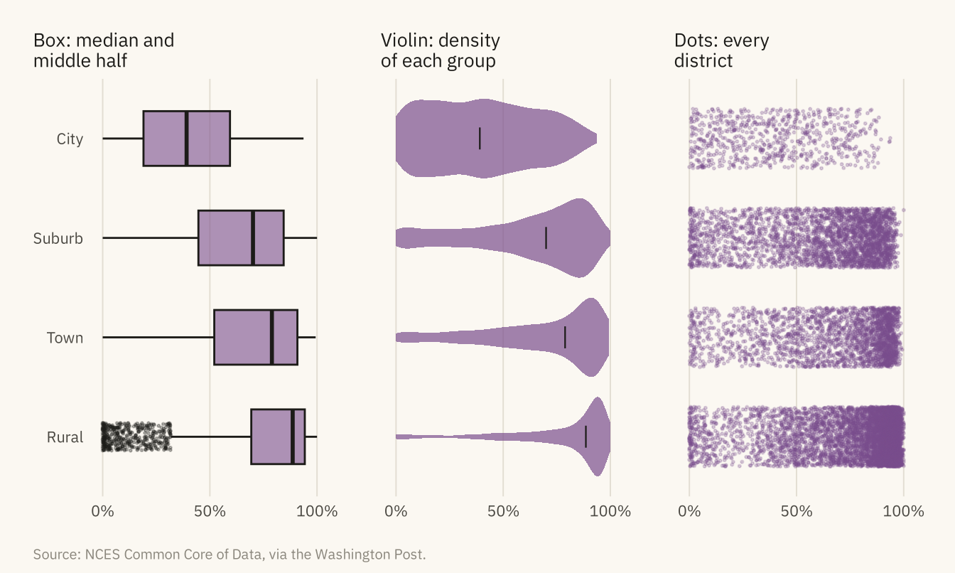
Figure 5.5
Share of Hispanic students by district in the fifteen states with the most districts, 2016-17, each drawn as a density and sorted by median. California and Texas have broad distributions reaching past 80 percent. New Jersey has a long tail. In the other twelve states, nearly every district is below 20 percent. Source: NCES Common Core of Data, via the Washington Post.
Code
states15 <- d17 |> count(state) |> slice_max(n, n = 15) |> pull(state)
rd <- d17 |> filter(state %in% states15) |>
  mutate(state = fct_reorder(state, hispanic, .fun = median))
ggplot(rd, aes(hispanic, state)) +
  geom_density_ridges(fill = mv_accent(), color = mv_ink$canvas, alpha = 0.85, scale = 2.2,
                      rel_min_height = 0.005, bandwidth = 3, linewidth = 0.4) +
  scale_x_continuous(labels = label_percent(scale = 1), limits = c(0, 100), expand = expansion(0)) +
  scale_y_discrete(expand = expansion(mult = c(0.02, 0.12))) +
  labs(title = "Share of Hispanic students by district, fifteen states, 2016-17",
       subtitle = "One density per state, sorted by median. The 15 states with the most districts.",
       x = NULL, y = NULL, caption = mv_source(src)) +
  theme_mv(grid = "x")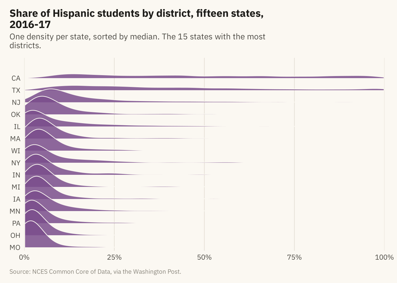
Figure 5.6
Cumulative share of districts by share of white students, 1994-95 and 2016-17. Read a value on the horizontal axis up to the curve to find the share of districts at or below it. The 2016-17 curve is above the earlier one at every point, which means more districts at every level of diversity. In 1994-95, 12 percent of districts were less than half white. In 2016-17, 22 percent were. The 1994-95 curve rises by 5 points at the right edge, where 642 districts reported no students of color. Source: NCES Common Core of Data, via the Washington Post.
Code
ec <- d |> mutate(year = factor(year, labels = c("1994-95", "2016-17")))
ggplot(ec, aes(white, color = year)) +
  stat_ecdf(linewidth = 1, pad = FALSE) +
  annotate("segment", x = 50, xend = 50, y = 0, yend = 0.225, color = mv_ink$mute, linewidth = 0.5, linetype = "22") +
  annotate("segment", x = 0, xend = 50, y = 0.118, yend = 0.118, color = mv_ink$mute, linewidth = 0.5, linetype = "22") +
  annotate("segment", x = 0, xend = 50, y = 0.225, yend = 0.225, color = mv_ink$mute, linewidth = 0.5, linetype = "22") +
  annotate("text", x = 4, y = 0.72, label = "Districts less than half white:\n22% in 2016-17\n12% in 1994-95",
           hjust = 0, vjust = 1, size = 3, family = mv_font(), color = mv_ink$ink, lineheight = 1) +
  scale_color_manual(values = c(`1994-95` = mv_ink$mute, `2016-17` = mv_accent()), name = NULL) +
  scale_x_continuous(labels = label_percent(scale = 1), expand = expansion(mult = c(0, 0.02))) +
  scale_y_continuous(labels = label_percent(), expand = expansion(mult = c(0, 0.04))) +
  labs(title = "Cumulative share of districts by share of white students, 1994-95 and 2016-17",
       subtitle = "Share of districts at or below each share of white students",
       x = "Share of white students in the district", y = "Share of districts",
       caption = mv_source(src)) +
  theme_mv()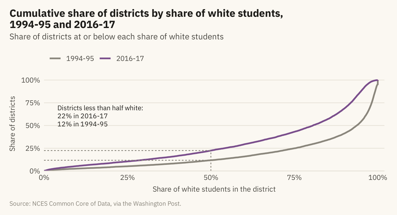
Figure 5.7
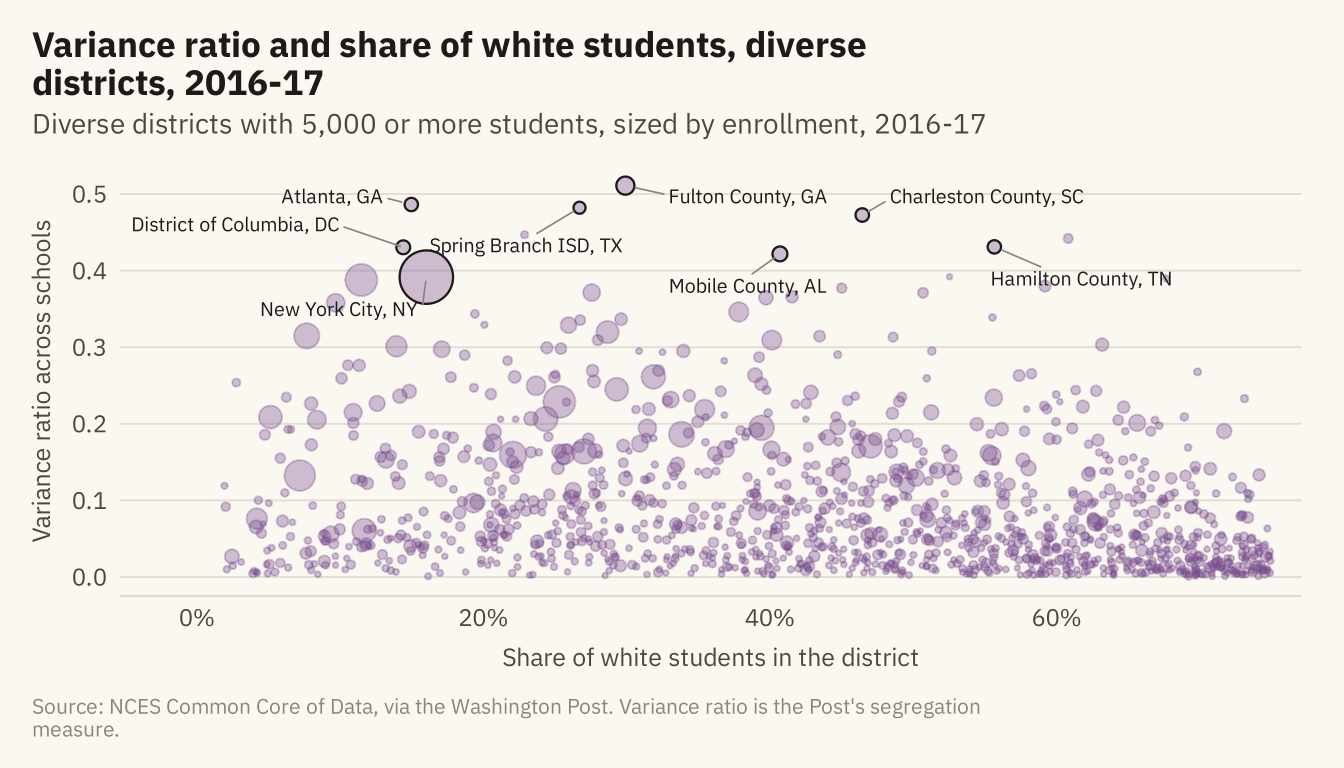
Districts classified as diverse in 2016-17, by the share of their students who are white and the variance ratio across their schools. A high ratio means students of different groups attend different schools within the same district. Named: the eight highest variance ratios among districts with 30,000 or more students. Source: NCES Common Core of Data, via the Washington Post.
Code
edges <- d17 |> filter(diversity == "Diverse", !is.na(variance_ratio), enrollment >= 5000)
named <- edges |> filter(enrollment >= 30000) |> slice_max(variance_ratio, n = 8) |>
  mutate(district = str_replace(district, " (Public Schools|School District|Independent School District|Schools|County Public Schools|Unified)$", ""),
         district = str_replace(district, " Isd$", " ISD"),
         district = str_replace(district, "^District Of Columbia$", "District of Columbia"),
         district = str_replace(district, "^Charleston 01$", "Charleston County"),
         district = paste0(district, ", ", state))
ggplot(edges, aes(white, variance_ratio)) +
  geom_point(aes(size = enrollment), color = mv_accent(), alpha = 0.35) +
  geom_point(data = named, aes(size = enrollment), color = mv_ink$ink, shape = 21, stroke = 0.6, fill = NA) +
  geom_text_repel(data = filter(named, state != "DC"), aes(label = district), size = 2.6, family = mv_font(), color = mv_ink$ink,
                  min.segment.length = 0, segment.color = mv_ink$mute, segment.size = 0.3, box.padding = 0.6,
                  point.padding = 0.4, force = 3, seed = 5, max.overlaps = 20) +
  geom_text_repel(data = filter(named, state == "DC"), aes(label = district), size = 2.6, family = mv_font(), color = mv_ink$ink,
                  min.segment.length = 0, segment.color = mv_ink$mute, segment.size = 0.3,
                  nudge_x = -11, nudge_y = 0.03, hjust = 1, seed = 5) +
  scale_size_area(max_size = 9, guide = "none") +
  scale_x_continuous(labels = label_percent(scale = 1), expand = expansion(mult = c(0.1, 0.03))) +
  labs(title = "Variance ratio and share of white students, diverse districts, 2016-17",
       subtitle = "Diverse districts with 5,000 or more students, sized by enrollment, 2016-17",
       x = "Share of white students in the district", y = "Variance ratio across schools",
       caption = mv_source(src, "Variance ratio is the Post's segregation measure")) +
  theme_mv()