# Where the data and the theme live. The defaults load from the companion
# site. Set MV_DATA and MV_THEME to local paths to work offline.
mv_data  <- Sys.getenv("MV_DATA",  "https://viz.marginoferrormedia.com/data")
mv_theme <- Sys.getenv("MV_THEME", "https://viz.marginoferrormedia.com/figures/mv-theme.R")Chapter 3: Reading a Chart Someone Else Made
The code behind every figure in Chapter 3 of Make It Visible, in the order the chapter draws them. Run the first chunk, then any figure. Each chunk stands on its own once the setup chunk has run.
Setup
Loads the theme, the packages, and the chapter’s data.
Code
source(mv_theme)
mv_set_chapter(3)
suppressPackageStartupMessages({ library(tidyverse); library(ggrepel); library(patchwork) })
us    <- read_csv(file.path(mv_data, "ch03-us-asylum.csv"), show_col_types = FALSE)
hosts <- read_csv(file.path(mv_data, "ch03-hosts-2022.csv"), show_col_types = FALSE)
us_year <- us |> group_by(year) |> summarise(refugees = sum(refugees), asylum = sum(asylum_seekers), .groups = "drop")
cap_theme <- theme(plot.caption = element_text(size = 7.5, hjust = 0, color = mv_ink$mute, family = mv_font()),
                   plot.background = element_rect(fill = mv_ink$canvas, color = NA))
plain_title <- theme(plot.title = element_text(size = rel(1), face = "plain"))
Figure 3.1
A chart of the kind that circulated during the immigration enforcement debate, redrawn from the UNHCR data it cited. The numbers are accurate. The unit is not stated, and the series counts pending claims rather than arrivals. Source: UNHCR Refugee Population Statistics Database.
Code
ggplot(us_year, aes(factor(year), asylum)) +
  geom_col(fill = "#C0392B", width = 0.75) +
  geom_text(data = filter(us_year, year %in% c(2010, 2022)),
            aes(label = label_comma()(asylum), hjust = c(0.2, 0.9)), vjust = -0.5, size = 3, family = mv_font(), fontface = "bold") +
  scale_y_continuous(labels = label_comma(), expand = expansion(mult = c(0, 0.15))) +
  labs(title = "ASYLUM SEEKERS IN THE U.S. UP 28,000% SINCE 2010",
       x = NULL, y = NULL, caption = "Source: UNHCR") +
  theme_mv(base_size = 10) +
  theme(plot.title = element_text(color = "#C0392B", size = rel(1.05)),
        axis.text.x = element_text(size = rel(0.8)))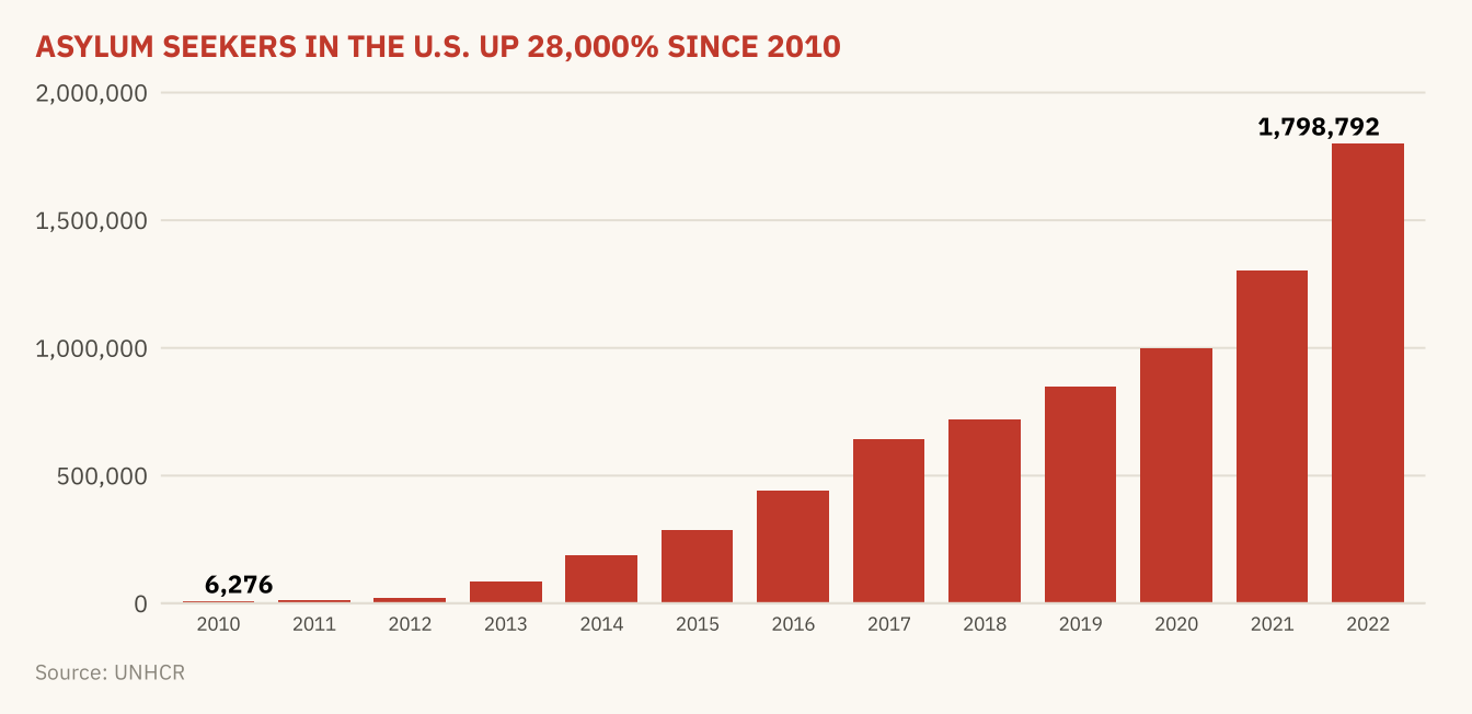
Figure 3.2
Asylum claims pending in the United States at the end of each year, 2010 to 2022. The series is a stock, not a count of arrivals. A backlog grows when claims are filed faster than they are decided, so the series depends on the speed of decisions as well as on arrivals. Source: UNHCR Refugee Population Statistics Database.
Code
ggplot(us_year, aes(year, asylum)) +
  geom_area(fill = mv_accent(), alpha = 0.15) +
  geom_line(color = mv_accent(), linewidth = 1) +
  geom_point(data = filter(us_year, year %in% c(2010, 2016, 2022)), color = mv_accent(), size = 2.2) +
  geom_text(data = filter(us_year, year %in% c(2010, 2016, 2022)),
            aes(label = label_comma(scale = 1e-3, suffix = "k", accuracy = 1)(asylum)),
            vjust = -0.9, size = 3, family = mv_font(), color = mv_ink$ink2) +
  scale_x_continuous(breaks = seq(2010, 2022, 3)) +
  scale_y_continuous(labels = label_comma(scale = 1e-3, suffix = "k"), limits = c(0, 2e6),
                     expand = expansion(mult = c(0.03, 0))) +
  labs(title = "Asylum claims pending in the United States, 2010 to 2022",
       subtitle = "Claims pending at the end of each year, in thousands",
       x = NULL, y = NULL, caption = mv_source("UNHCR Refugee Population Statistics Database")) +
  theme_mv()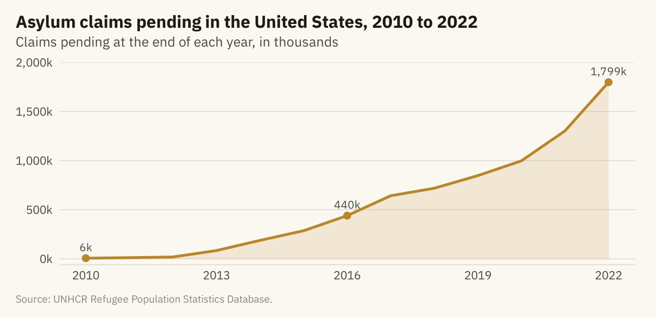
Figure 3.3
Refugees hosted by the United States, 2010 to 2022. Left, the axis starts at 250,000, and the bars appear to rise about eightfold. Right, the axis starts at zero, and the rise is 37 percent. Source: UNHCR Refugee Population Statistics Database.
Code
tr <- ggplot(us_year, aes(year, refugees)) +
  geom_col(fill = mv_accent(), width = 0.7) +
  coord_cartesian(ylim = c(250000, 370000)) +
  scale_x_continuous(breaks = c(2010, 2016, 2022)) +
  scale_y_continuous(labels = label_comma()) +
  labs(x = NULL, y = NULL, title = "Axis starts at 250,000") + theme_mv(base_size = 10) + plain_title
zr <- ggplot(us_year, aes(year, refugees)) +
  geom_col(fill = mv_accent(), width = 0.7) +
  scale_x_continuous(breaks = c(2010, 2016, 2022)) +
  scale_y_continuous(labels = label_comma(), limits = c(0, 400000), expand = expansion(0)) +
  labs(x = NULL, y = NULL, title = "Axis starts at zero") + theme_mv(base_size = 10) + plain_title
tr + zr + plot_annotation(caption = mv_source("UNHCR Refugee Population Statistics Database"), theme = cap_theme)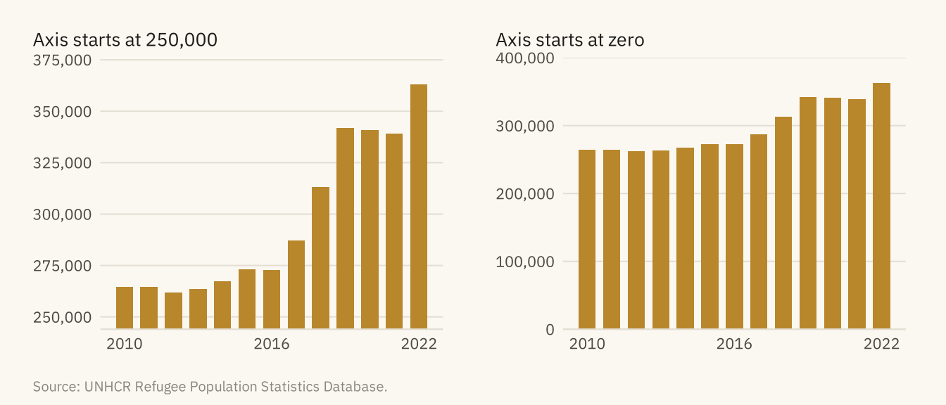
Figure 3.4
Refugees hosted by the United States, drawn over three time windows. From 2010 to 2022, the series rises 37 percent. From 2019 to 2021, it falls 1 percent. From 2021 to 2022, it rises 7 percent. Each panel has its own vertical axis, and none starts at zero. The middle axis spans 4,000 people, so a fall of 2,500 fills the panel. The direction and the apparent size of the trend both depend on choices the author made. Source: UNHCR Refugee Population Statistics Database.
Code
win <- function(from, to, title, lo, hi, step) {
  d <- filter(us_year, year >= from, year <= to)
  ggplot(d, aes(year, refugees)) +
    geom_line(color = mv_accent(), linewidth = 0.9) + geom_point(color = mv_accent(), size = 1.8) +
    scale_x_continuous(breaks = c(from, to)) +
    scale_y_continuous(labels = label_comma(), limits = c(lo, hi), breaks = seq(lo, hi, step),
                       expand = expansion(0)) +
    labs(x = NULL, y = NULL, title = title) + theme_mv(base_size = 10) + plain_title +
    theme(axis.text.y = element_text(size = rel(0.75)))
}
win(2010, 2022, "2010 to 2022: up 37%", 250000, 375000, 25000) +
  win(2019, 2021, "2019 to 2021: down 1%", 338000, 342000, 1000) +
  win(2021, 2022, "2021 to 2022: up 7%", 335000, 365000, 5000) +
  plot_annotation(caption = mv_source("UNHCR Refugee Population Statistics Database"), theme = cap_theme)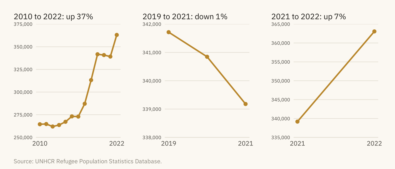
Figure 3.5
Refugees and asylum seekers hosted in 2022. Left, the ten countries hosting the largest numbers. Right, the ten with the most hosted per 1,000 residents, among countries with over one million people. Only Türkiye and Iran appear on both lists. Source: UNHCR; population from Natural Earth estimates.
Code
top_n <- hosts |> slice_max(hosted, n = 10) |> mutate(asylum = fct_reorder(str_replace(asylum, " \\(.*\\)", ""), hosted))
top_r <- hosts |> filter(pop_est > 1e6) |> slice_max(per_1000, n = 10) |>
  mutate(asylum = fct_reorder(str_replace(asylum, " \\(.*\\)", ""), per_1000))
both <- intersect(as.character(top_n$asylum), as.character(top_r$asylum))

p1 <- ggplot(top_n, aes(hosted, asylum, fill = asylum %in% both)) +
  geom_col(width = 0.7) +
  scale_fill_manual(values = c(`FALSE` = mv_ink$mute, `TRUE` = mv_accent()), guide = "none") +
  scale_x_continuous(labels = label_comma(scale = 1e-6, suffix = "M"), expand = expansion(mult = c(0, 0.05))) +
  labs(x = NULL, y = NULL, title = "By count: people hosted") + theme_mv(base_size = 10, grid = "x") + plain_title
p2 <- ggplot(top_r, aes(per_1000, asylum, fill = asylum %in% both)) +
  geom_col(width = 0.7) +
  scale_fill_manual(values = c(`FALSE` = mv_ink$mute, `TRUE` = mv_accent()), guide = "none") +
  scale_x_continuous(breaks = seq(0, 100, 25), expand = expansion(mult = c(0, 0.05))) +
  labs(x = NULL, y = NULL, title = "By rate: hosted per 1,000 residents") + theme_mv(base_size = 10, grid = "x") + plain_title
p1 + p2 + plot_annotation(subtitle = "Gold bars: countries on both lists",
                          caption = mv_source("UNHCR; Natural Earth population estimates"),
                          theme = cap_theme + theme(plot.subtitle = element_text(size = 9, color = mv_ink$ink2, family = mv_font())))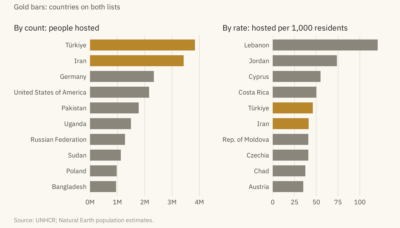
Figure 3.6
Refugees and pending asylum claims in the United States on a dual-axis chart (left) and as two panels with their own scales (right). On the dual axis, the lines cross in 2016. The crossing exists only because of how the two scales were chosen. Source: UNHCR Refugee Population Statistics Database.
Code
k <- 1.6
dual <- ggplot(us_year, aes(year)) +
  geom_line(aes(y = refugees), color = mv_ink$ink, linewidth = 0.9) +
  geom_line(aes(y = asylum / k), color = mv_accent(), linewidth = 0.9) +
  scale_y_continuous(name = "Refugees", labels = label_comma(scale = 1e-3, suffix = "k"),
                     limits = c(0, NA),
                     sec.axis = sec_axis(~ . * k, name = "Asylum claims pending",
                                         breaks = seq(0, 1.8e6, 3e5),
                                         labels = label_comma(scale = 1e-3, suffix = "k"))) +
  scale_x_continuous(breaks = c(2010, 2016, 2022)) +
  labs(x = NULL, title = "Dual axis: refugees left, pending claims right") +
  theme_mv(base_size = 10) + plain_title +
  theme(axis.title.y.left = element_text(color = mv_ink$ink), axis.title.y.right = element_text(color = mv_accent()))
long <- us_year |> pivot_longer(-year, names_to = "series", values_to = "n") |>
  mutate(series = recode(series, refugees = "Refugees", asylum = "Asylum claims pending"))
facets <- ggplot(long, aes(year, n, color = series)) +
  geom_line(linewidth = 0.9) +
  facet_wrap(~ series, ncol = 1, scales = "free_y") +
  scale_color_manual(values = c(`Refugees` = mv_ink$ink, `Asylum claims pending` = mv_accent()), guide = "none") +
  scale_x_continuous(breaks = c(2010, 2016, 2022)) +
  scale_y_continuous(labels = label_comma(scale = 1e-3, suffix = "k"), limits = c(0, NA)) +
  labs(x = NULL, y = NULL, title = "Two panels: each from zero") + theme_mv(base_size = 10) + plain_title
dual + facets + plot_annotation(caption = mv_source("UNHCR Refugee Population Statistics Database"), theme = cap_theme)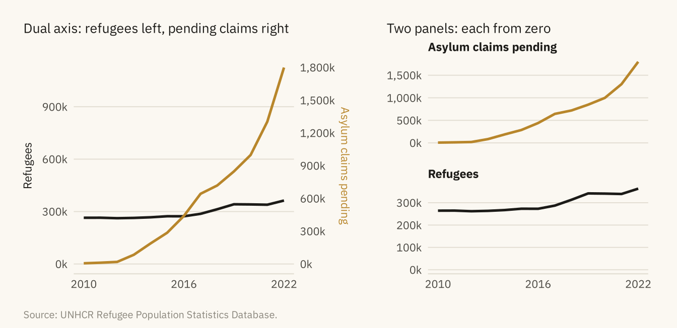
Figure 3.7
Pending asylum claims in the United States by country of origin. Top, a stacked area with eight countries. Only the bottom layer can be read accurately. Bottom, the same eight countries as small multiples sharing one scale. Each series can be read on its own and compared with the others. Source: UNHCR Refugee Population Statistics Database.
Code
top8 <- us |> filter(year == 2022) |> slice_max(asylum_seekers, n = 8) |> pull(origin)
orig <- us |> filter(origin %in% top8) |>
  mutate(origin = str_replace(origin, " \\(.*\\)", ""),
         origin = fct_reorder(origin, -asylum_seekers, .fun = last))
stack <- ggplot(orig, aes(year, asylum_seekers, fill = origin)) +
  geom_area(color = mv_ink$canvas, linewidth = 0.3) +
  scale_fill_manual(values = colorRampPalette(c("#D6C79C", mv_accent(), "#3A1F05"))(8)) +
  scale_x_continuous(breaks = c(2010, 2016, 2022)) +
  scale_y_continuous(labels = label_comma(scale = 1e-3, suffix = "k"), expand = expansion(0)) +
  labs(x = NULL, y = NULL, fill = NULL, title = "Stacked area: eight origin countries") +
  guides(fill = guide_legend(nrow = 2)) +
  theme_mv(base_size = 10) + plain_title +
  theme(legend.text = element_text(size = rel(0.72)), legend.key.size = unit(0.6, "lines"))
small <- ggplot(orig, aes(year, asylum_seekers)) +
  geom_area(fill = mv_accent(), alpha = 0.2) +
  geom_line(color = mv_accent(), linewidth = 0.7) +
  facet_wrap(~ origin, ncol = 4) +
  scale_x_continuous(breaks = c(2010, 2022)) +
  scale_y_continuous(labels = label_comma(scale = 1e-3, suffix = "k"), expand = expansion(mult = c(0, 0.05))) +
  labs(x = NULL, y = NULL, title = "Small multiples: one panel per country") +
  theme_mv(base_size = 10) + plain_title + theme(strip.text = element_text(size = rel(0.8)))
(stack / small) + plot_layout(heights = c(1, 1.1)) +
  plot_annotation(caption = mv_source("UNHCR Refugee Population Statistics Database"), theme = cap_theme)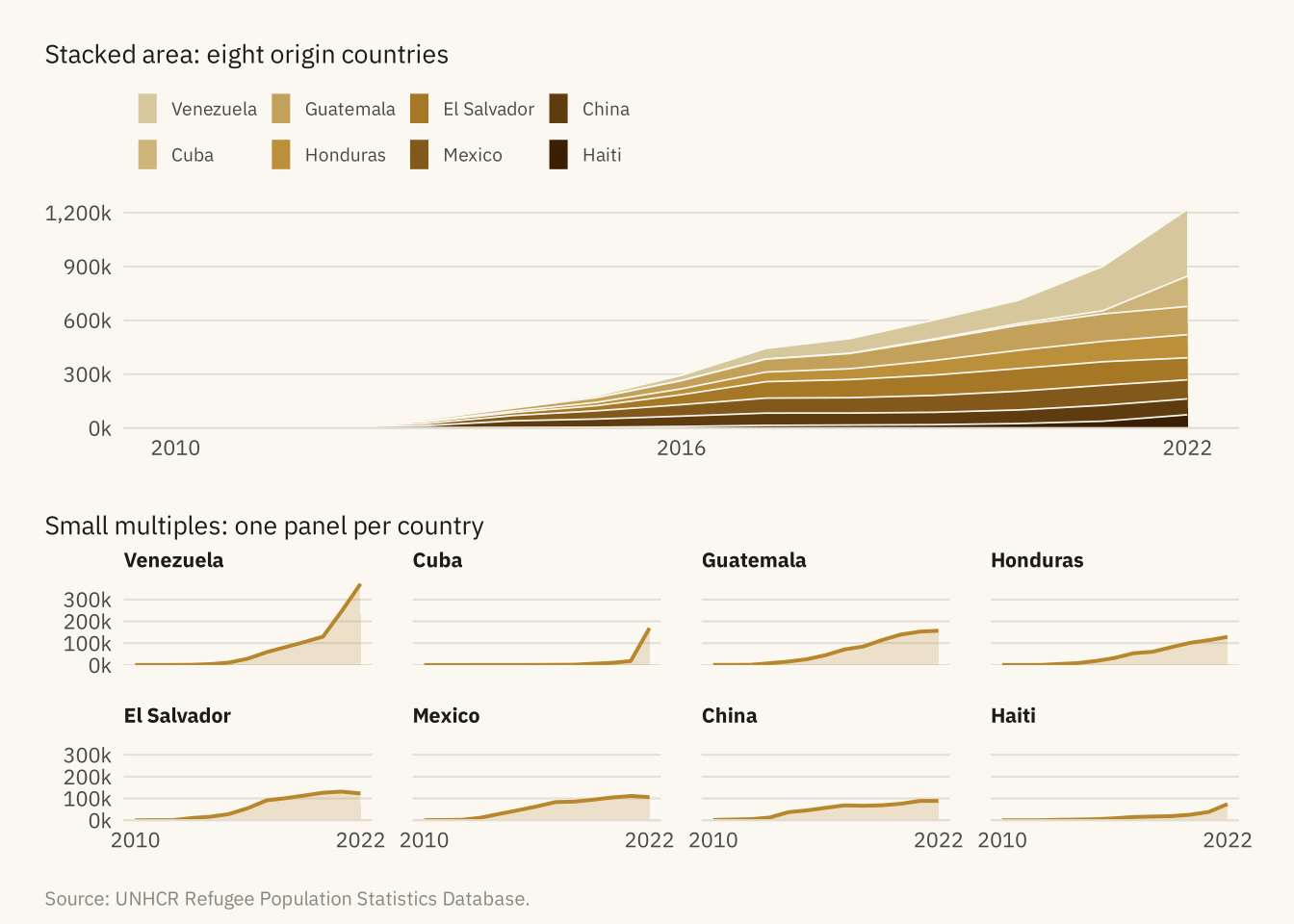
The reading protocol. Seven questions, in the order to ask t
Code
tibble::tribble(
  ~Question, ~`What to look for`, ~`What it caught in the viral chart`,
  "1. What is being counted?", "The unit. Stock or flow. Count or rate.", "A backlog read as arrivals",
  "2. Where does the axis start?", "The lowest axis value. Zero for bars.", "Nothing. The bars start at zero",
  "3. What is the time window?", "Start and end dates, and what the full series shows.", "Nothing. 2010 is where the data starts",
  "4. What is the denominator?", "Per person, per capita, per year, or none.", "No denominator. The US is 4th by count, far down by rate",
  "5. Does the encoding fit?", "Dual axes, stacks, pies, 3D, rainbow scales.", "Nothing. Bars from zero",
  "6. What comparison is invited?", "The title and highlight. What comparison is absent.", "2022 against 2010, with no comparison to decisions or other hosts",
  "7. Who made it, and why?", "Source line, author, purpose.", "One series cut from a fuller picture and given a headline"
) |> knitr::kable()| Question | What to look for | What it caught in the viral chart |
|---|---|---|
| 1. What is being counted? | The unit. Stock or flow. Count or rate. | A backlog read as arrivals |
| 2. Where does the axis start? | The lowest axis value. Zero for bars. | Nothing. The bars start at zero |
| 3. What is the time window? | Start and end dates, and what the full series shows. | Nothing. 2010 is where the data starts |
| 4. What is the denominator? | Per person, per capita, per year, or none. | No denominator. The US is 4th by count, far down by rate |
| 5. Does the encoding fit? | Dual axes, stacks, pies, 3D, rainbow scales. | Nothing. Bars from zero |
| 6. What comparison is invited? | The title and highlight. What comparison is absent. | 2022 against 2010, with no comparison to decisions or other hosts |
| 7. Who made it, and why? | Source line, author, purpose. | One series cut from a fuller picture and given a headline |
Figure 3.8
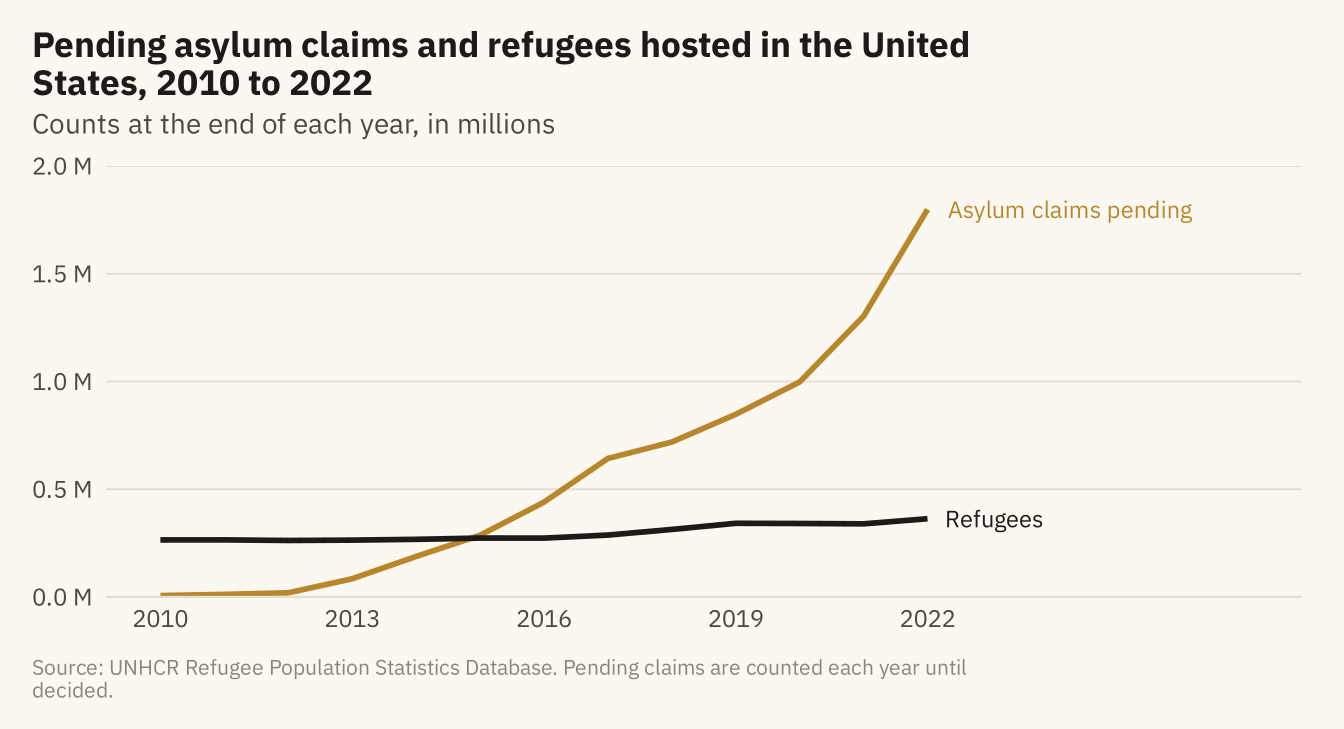
Pending asylum claims and refugees hosted in the United States, 2010 to 2022, with the unit stated and both series from zero. The backlog grew from 6,000 to 1.8 million. The refugee series, which the viral chart left out, grew slowly over the same years. Source: UNHCR Refugee Population Statistics Database.
Code
ends <- long |> filter(year == 2022)
ggplot(long, aes(year, n, color = series)) +
  geom_line(linewidth = 1) +
  mv_label_end(ends, aes(label = series, color = series), nudge_x = 0.3) +
  scale_color_manual(values = c(`Refugees` = mv_ink$ink, `Asylum claims pending` = mv_accent()), guide = "none") +
  scale_x_continuous(breaks = seq(2010, 2022, 3), limits = c(2010, 2027)) +
  scale_y_continuous(labels = label_comma(scale = 1e-6, suffix = " M"), limits = c(0, 2e6), expand = expansion(0)) +
  labs(title = "Pending asylum claims and refugees hosted in the United States, 2010 to 2022",
       subtitle = "Counts at the end of each year, in millions",
       x = NULL, y = NULL, caption = mv_source("UNHCR Refugee Population Statistics Database",
       "Pending claims are counted each year until decided")) +
  theme_mv()